
CHAPTER 5
Dimension tables provide the context for fact tables and hence for all the measurements presented in the data warehouse. Although dimension tables are usually much smaller than fact tables, they are the heart and soul of the data warehouse because they provide entry points to data. We often say that a data warehouse is only as good as its dimensions. We think the main mission of the ETL team is the handoff of the dimension tables and the fact tables in the delivery step, leveraging the end user applications most effectively.
PROCESS CHECK Planning & Design:
Requirements/Realities → Architecture → Implementation → Test/Release
Data Flow: Extract → Clean → Conform → Deliver
Chapters 5 and 6 are the pivotal elements of this book; they describe in a highly disciplined way how to deliver data to end users and their analytic applications. While there is considerable variability in the data structures and delivery-processing techniques leading up to this handoff, the final ETL step of preparing the dimensional table structures is much more constrained and disciplined.
Please keep in mind that our insistence on using these highly constrained design techniques is not adherence to a foolish consistency of a dimensional modeling methodology but rather is the key to building data warehouse systems with replicable, scalable, usable, and maintainable architectures. The more a data warehouse design deviates from these standardized dimensional modeling techniques, the more it becomes a custom programming job. Most IT developers are clever enough to take on a custom programming job, and most find such development to be intellectually stimulating. But custom programming is the kiss of death for building replicable, scalable, usable, and maintainable systems.
The Basic Structure of a Dimension
All dimensions should be physically built to have the minimal set of components shown in Figure 5.1. The primary key is a single field containing a meaningless, unique integer. We call a meaningless integer key a surrogate. The data warehouse ETL process should always create and insert the surrogate keys. In other words, the data warehouse owns these keys and never lets another entity assign them.
Figure 5.1 The basic structure of a dimension.

The primary key of a dimension is used to join to fact tables. Since all fact tables must preserve referential integrity, the primary dimension key is joined to a corresponding foreign key in the fact table. This is shown in our insurance example in Figure 2.3 in Chapter 2. We get the best possible performance in most relational databases when all joins between dimension tables and fact tables are based on these single field integer joins. And finally, our fact tables are much more compact when the foreign key fields are simple integers.
All dimension tables should possess one or more other fields that compose the natural key of the dimension. We show this in Figure 5.1 as an ID and designate the natural key field(s) with NK. The natural key is not a meaningless surrogate quantity but rather is based on one or more meaningful fields extracted from the source system. For instance, a simple static (nonchanging) employee dimension would probably have the familiar EMP_ID field, which is probably the employee number assigned by the human resources production system. EMP_ID would be the natural key of this employee dimension. We still insist on assigning a data warehouse surrogate key in this case, because we must insulate ourselves from weird administrative steps that an HR system might take. For instance, in the future we might have to merge in bizarrely formatted EMP_IDs from another HR system in the event of an acquisition.
When a dimension is static and is not being updated for historical changes to individual rows, there is a 1-to-1 relationship between the primary surrogate key and the natural key. But we will see a little later in this chapter that when we allow a dimension to change slowly, we generate many primary surrogate keys for each natural key as we track the history of changes to the dimension. In other words, in a slowly changing dimension, the relationship between the primary surrogate key and the natural key is many-to-1. In our employee dimension example, each of the changing employee profile snapshots would have different and unique primary surrogate keys, but the profiles for a given employee would all have the same natural key (EMP_ID). This logic is explained in detail in the section on slowly changing dimensions in this chapter.
The final component of all dimensions, besides the primary key and the natural key, is the set of descriptive attributes. Descriptive attributes are predominately textual, but numeric descriptive attributes are legitimate. The data warehouse architect probably will specify a very large number of descriptive attributes for dimensions like employee, customer, and product. Do not be alarmed if the design calls for 100 descriptive attributes in a dimension! Just hope that you have clean sources for all these attributes. More on this later.
The data warehouse architect should not call for numeric fields in a dimension that turn out to be periodically measured quantities. Such measured quantities are almost certainly facts, not descriptive attributes. All descriptive attributes should be truly static or should only change slowly and episodically. The distinction between a measured fact and a numeric descriptive attribute is not as difficult as it sounds. In 98 percent of the cases, the choice is immediately obvious. In the remaining two percent, pretty strong arguments can be made on both sides for modeling the quantity either as a fact or as a dimensional attribute. For instance, the standard (catalog) price of a product is a numeric quantity that takes on both roles. In the final analysis, it doesn’t matter which choice is made. The requesting applications will look different depending on where this numeric quantity is located, but the information content will be the same. The difference between these two choices will start to become important if it turns out that the standard price is actually slowly changing. As the pace of the change accelerates, modeling the numeric quantity as a measured fact becomes more attractive.
 Generating Surrogate Keys for Dimensions
Creating surrogate keys via the DBMS is probably the most common technique used today. However, we see this trend changing. In the past, it was common practice to have surrogate keys created and inserted by database triggers. Subsequently, it has been determined that triggers cause severe bottlenecks in the ETL process and should be eliminated from any new processes being created. Even though it is still acceptable for the integers for a surrogate key to be maintained by the DBMS, these integers should be called by the ETL process directly. Having the ETL process call the database sequence will produce a significant improvement in ETL performance over the use of database triggers.
Also, using the database to generate surrogate keys almost guarantees that the keys will be out of sync across the different environments of the data warehouse— development, test, and production. As each environment gets loaded at different intervals, their respective database could generates different surrogate key values for the same incoming dimension records. This lack of synchronization will cause confusion during testing for developers and users alike.
For ultimate efficiency, consider having an ETL tool or third-party application generate and maintain your surrogate keys. Make sure that efficient generation and maintenance of surrogate keys are in your ETL proof-of-concept success criteria.
A tempting solution seen repeatedly during design reviews is concatenating the natural key of the source system and a date stamp that reflects when the record was either created in the source system or inserted into the data warehouse. Giving the surrogate key intelligence—the exact time of its creation—may be useful in some situations, but it is not an acceptable alternative to a true integer-based surrogate key. Intelligent or smart keys fail as an acceptable surrogate key for the following reasons:
 By definition. Surrogate keys, by definition, are supposed to be meaningless. By applying intelligence to the surrogate key, their responsibility is broadened, making them need to be maintained. What happens if a primary key in the source system changes—or gets corrected in some way? The concatenated smart key would need to be updated, as will all of its associated records in fact tables throughout the entire data warehouse.
Performance. Concatenating the source system key with a date stamp degrades query performance. As part of the data warehouse team, you have no control over the content of source system keys and must be able to handle any data type. This fact forces you to use the CHAR or VARCHAR data types to accommodate alpha, numeric, or alphanumeric keys coming from the source systems. Moreover, by appending the date stamp to the key, potentially 16 characters or more, the field can become unwieldy. What’s worse, this key will need to be propagated into huge fact tables throughout the entire warehouse. The space to store the data and indexes would be excessive, causing ETL and end user query performance to diminish. Additionally, joining these large VARCHAR concatenated columns during query time will be slow when compared to the same join using INTEGER columns.
Data type mismatch. Veteran data warehouse data modelers will know to build the dimensional model surrogate keys with the NUMBER or INTEGER data type. This data type prevents alpha characters from being inserted, thwarting the use of the concatenated date stamp method.
Dependency on source system. The use of the smart-key approach is dependent on the source system revealing exactly when an attribute in a dimension changed. In many cases, this information is simply not available. Without reliable maintenance of some kind of audit columns, attaining the exact timestamp of a change can be impossible.
Heterogeneous sources. The concatenation of the natural key and date stamp supports only a homogeneous environment. In virtually all enterprise data warehouses, common dimensions are sourced by many different source systems. These source systems each have their own purpose and can uniquely identify the same values of a dimension differently. The concatenated natural key, date-stamp approach falls short with the introduction of a second source system. Natural keys from each system must be stored equally, in dedicated nonkey columns in the dimension. Imagine attempting to concatenate each natural key and their respective timestamps—a maintenance nightmare.
The attractive characteristic of using this forbidden smart-key strategy is its simplicity at ETL development time when building the first data mart, when it is quite simple to implement a smart key by appending the SYSDATE to the natural key upon insertion. Avoid the temptation of this prohibited shortcut. This approach doesn’t scale to your second data mart.
The Grain of a Dimension
Dimensional modelers frequently refer to the grain of a dimension. By this they mean the definition of the key of the dimension, in business terms. It is then a challenge for the data warehouse architect and the ETL team to analyze a given data source and make sure that a particular set of fields in that source corresponds to the definition of the grain. A common and notorious example is the commercial customer dimension. It is easy to say that the grain of the dimension is the commercial customer. It is often quite another thing to be absolutely sure that a given source file always implements that grain with a certain set of fields. Data errors and subtleties in the business content of a source file can violate your initial assumptions about the grain. Certainly, a simple test of a source file to demonstrate that fields A, B, and C implement the key to the candidate dimension table source is the query:
Select A, B, C, count(*)
From dimensiontablesource
Group by A, B, C Having Count(*) > 1
If this query returns any rows, the fields A, B, and C do not implement the key (and hence the grain) of this dimension table. Furthermore, this query is obviously useful, because it directs you to exactly the rows that violate your assumptions.
It’s possible that the extract process itself can be the culprit for exploding the rows being extracted, creating duplicates. For example, in a denormalized Orders transaction system, instead of referring to a source table that stores the distinct Ship Via values for the Order, the textual values of the attribute may very well be stored repeatedly directly in the Orders transaction table. To create the dimensional model, you build the Ship Via dimension by performing a SELECT DISTINCT on the Orders table. Any data anomalies in the original Orders table will create bogus duplicate entries in the Ship Via dimension.
The Basic Load Plan for a Dimension
A few dimensions are created entirely by the ETL system and have no real outside source. These are usually small lookup dimensions where an operational code is translated into words. In these cases, there is no real ETL processing. The little lookup dimension is simply created directly as a relational table in its final form.
But the important case is the dimension extracted from one or more outside sources. We have already described the four steps of the ETL data flow thread in some detail. Here are a few more thoughts relating to dimensions specifically.
Dimensional data for the big, complex dimensions like customer, supplier, or product is frequently extracted from multiple sources at different times. This requires special attention to recognizing the same dimensional entity across multiple source systems, resolving the conflicts in overlapping descriptions, and introducing updates to the entities at various points. These topics are handled in this chapter.
Data cleaning consists of all the steps required to clean and validate the data feeding a dimension and to apply known business rules to make the data consistent. For some simple, smaller dimensions, this module may be almost nonexistent. But for the big important dimensions like employee, customer, and product, the data-cleaning module is a very significant system with many subcomponents, including column validity enforcement, cross-column value checking, and row deduplication.
Data conforming consists of all the steps required to align the content of some or all of the fields in the dimension with fields in similar or identical dimensions in other parts of the data warehouse. For instance, if we have fact tables describing billing transactions and customer-support calls, they probably both have a customer dimension. In large enterprises, the original sources for these two customer dimensions could be quite different. In the worst case, there could be no guaranteed consistency between fields in the billing-customer dimension and the support-customer dimension. In all cases where the enterprise is committed to combining information across multiple sources, like billing and customer support, the conforming step is required to make some or all of the fields in the two customer dimensions share the same domains. We describe the detailed steps of conforming dimensions in the Chapter 4. After the conforming step has modified many of the important descriptive attributes in the dimension, the conformed data is staged again.
Finally, the data-delivering module consists of all the steps required to administer slowly changing dimensions (SCDs, described in this chapter) and write the dimension to disk as a physical table in the proper dimensional format with correct primary keys, correct natural keys, and final descriptive attributes. Creating and assigning the surrogate keys occur in this module. This table is definitely staged, since it is the object to be loaded into the presentation system of the data warehouse. The rest of this chapter describes the details of the data-delivering module in various situations.
Flat Dimensions and Snowflaked Dimensions
PROCESS CHECK Planning & Design:
Requirements/Realities → Architecture → Implementation → Test/Release
Data Flow: Extract → Clean → Conform → Deliver
Dimension tables are denormalized flat tables. All hierarchies and normalized structures that may be present in earlier staging tables should be flattened in the final step of preparing the dimension table, if this hasn’t happened already. All attributes in a dimension must take on a single value in the presence of the dimension’s primary key. Most of the attributes will be of medium and low cardinality. For instance, the gender field in an employee dimension will have a cardinality of three (male, female, and not reported), and the state field in a U.S. address will have a cardinality of 51 (50 states plus Washington, DC). If earlier staging tables are in third normal form, these flattened second normal form dimension tables are easily produced with a simple query against the third normal form source. If all the proper data relationships have been enforced in the data-cleaning step, these relationships are preserved perfectly in the flattened dimension table. This point is consistently misunderstood by proponents of delivering data to end users via a normalized model. In the dimensional-modeling world, the data-cleaning step is separated from the data-delivery step, in such a way that all proper data relationships are delivered to the end user, without the user needing to navigate the complex normalized structures.
It is normal for a complex dimension like store or product to have multiple simultaneous, embedded hierarchical structures. For example, the store dimension could have a normal geographic hierarchy of location, city, county, and state and also have a merchandising-area hierarchy of location, district, and region. These two hierarchies should coexist in the same store dimension. All that is required is that every attribute be single valued in the presence of the dimension table’s primary key.
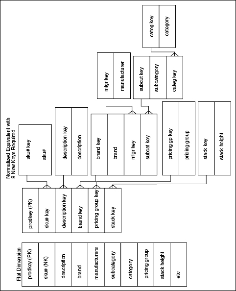
If a dimension is normalized, the hierarchies create a characteristic structure known as a snowflake, if indeed the levels of the hierarchies obey perfect many-to-1 relationships. See Figure 5.2. It is important to understand that there is no difference in the information content between the two versions of dimensions in this figure. The difference we do care about is the negative impact the normalized, snowflaked model has on the end user environment. There are two problems. First, if the strict many-to-1 relationships in a hierarchical model change, the normalized table schema and the declared joins between the tables must change, and the end user environment must be recoded at some level for applications to continue working. Flat versions of the dimension do not have this problem. Second, complex schemas are notorious for confusing end users, and a normalized schema requires masking this complexity in the presentation area of the data warehouse. Generally, flat dimension tables can appear directly in user interfaces with less confusion.
Figure 5.2 Flat and snowflaked versions of a dimension.
Having railed against snowflaked dimensions, there are nevertheless some situations where a kind of snowflaking is recommended. These are best described as subdimensions of another dimension. Please refer to the section with this name later in this chapter.
If an attribute takes on multiple values in the presence of the dimension’s primary key, the attribute cannot be part of the dimension. For example, in a retail-store dimension, the cash register ID attribute takes on many values for each store. If the grain of the dimension is the individual store, the cash register ID cannot be an attribute in that dimension. To include the cash register attribute, the grain of the dimension must be redeclared to be cash register, not store. But since cash registers roll up to stores in a perfect many-to-1 relationship, the new cash-register dimension contains all of the store attributes, since they are all single valued at the cash-register level.
Each time a new dimension record is created, a fresh surrogate key must be assigned. See Figure 5.3. This meaningless integer is the primary key of the dimension. In a centralized data warehouse environment, the surrogate keys for all dimensions could be generated from a single source. In that case, a master metadata element contains the highest key used for all the dimensions simultaneously. However, even in a highly centralized data warehouse, if there are enough simultaneous ETL jobs running, there could be contention for reading and writing this single metadata element. And of course, in a distributed environment, this approach doesn’t make much sense. For these reasons, we recommend that a surrogate key counter be established for each dimension table separately. It doesn’t matter whether two different surrogate keys have the same numeric value; the data warehouse will never confuse the separate dimensional domains, and no application ever analyzes the value of a surrogate key, since by definition it is meaningless.
Figure 5.3 Assigning the surrogate key in the dimensionalizing step.

Date and Time Dimensions
PROCESS CHECK Planning & Design:
Requirements/Realities → Architecture → Implementation → Test/Release
Data Flow: Extract → Clean → Conform → Deliver
Virtually every fact table has one or more time-related dimension foreign keys. Measurements are defined at specific points and most measurements are repeated over time.
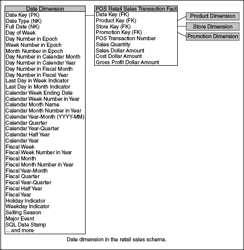
The most common and useful time dimension is the calendar date dimension with the granularity of a single day. This dimension has surprisingly many attributes, as shown in Figure 5.4. Only a few of these attributes (such as month name and year) can be generated directly from an SQL date-time expression. Holidays, work days, fiscal periods, week numbers, last day of month flags, and other navigational attributes must be embedded in the calendar date dimension and all date navigation should be implemented in applications by using the dimensional attributes. The calendar date dimension has some very unusual properties. It is one of the only dimensions
Figure 5.4 Attributes needed for a calendar date dimension.
completely specified at the beginning of the data warehouse project. It also doesn’t have a conventional source. The best way to generate the calendar date dimension is to spend an afternoon with a spreadsheet and build it by hand. Ten years worth of days is fewer than 4000 rows.
Every calendar date dimension needs a date type attribute and a full date description attribute as depicted in Figure 5.4. These two fields compose the natural key of the table. The date type attribute almost always has the value date, but there must be at least one record that handles the special nonapplicable date situation where the recorded date is inapplicable, corrupted, or hasn’t happened yet. Foreign key references in fact tables referring to these special data conditions must point to a nondate date in the calendar date table! You need at least one of these special records in the calendar date table, but you may want to distinguish several of these unusual conditions. For the inapplicable date case, the value of the date type is inapplicable or NA. The full date attribute is a full relational date stamp, and it takes on the legitimate value of null for the special cases described previously. Remember that the foreign key in a fact table can never be null, since by definition that violates referential integrity.
The calendar date primary key ideally should be a meaningless surrogate key, but many ETL teams can’t resist the urge to make the key a readable quantity such as 20040718, meaning July 18, 2004. However, as with all smart keys, the few special records in the time dimension will make the designer play tricks with the smart key. For instance, the smart key for the inapplicable date would have to be some nonsensical value like 99999999, and applications that tried to interpret the date key directly without using the dimension table would always have to test against this value because it is not a valid date.
Even if the primary surrogate key of the calendar date dimension table is a true meaningless integer, we recommend assigning date surrogate keys in numerical order and using a standard starting date for the key value of zero in every date dimension table. This allows any fact table with a foreign key based on the calendar date to be physically partitioned by time. In other words, the oldest data in a fact table could be on one physical medium, and the newest data could be on another. Partitioning also allows the DBA to drop and rebuild indexes on just the most recent data, thereby making the loading process faster, if only yesterday’s data is being loaded. Finally, the numeric value of the surrogate key for the special inapplicable time record should probably be a high number so that the inapplicable time-stamped records are in the most active partition. This assumes that these fact records are more likely to be rewritten in an attempt to correct data.
Although the calendar date dimension is the most important time dimension, we also need a calendar month dimension when the fact table’s time grain is a month. In some environments, we may need to build calendar week, quarter, or year dimensions as well if there are fact tables at each of these grains. The calendar month dimension should be a separate physical table and should be created by physically eliminating selected rows and columns from the calendar day dimension. For example, either the first or the last day of each month could be chosen from the day dimension to be the basis of the month dimension. It is possible to define a view on a calendar day dimension that implements a calendar month dimension, but this is not recommended. Such a view would drag a much larger table into every month-based query than if the month table were its own physical table. Also, while this view technique can be made to work for calendar dimensions, it cannot be made to work for dimensions like customer or product, since individual customers and products come and go. Thus, you couldn’t build a brand table with a view on the base product table, for instance, because you wouldn’t know which individual product to choose to permanently represent a brand.
In some fact tables, time is measured below the level of calendar day, down to minute or even second. One cannot build a time dimension with every minute or every second represented. There are more than 31 million seconds in a year! We want to preserve the powerful calendar date dimension and simultaneously support precise querying down to the minute or second. We may also want to compute very precise time intervals by comparing the exact time of two fact table records. For these reasons, we recommend the design shown in Figure 5.5. The calendar day component of the precise time remains as a foreign key reference to our familiar calendar day dimension. But we also embed a full SQL date-time stamp directly in the fact table for all queries requiring the extra precision. Think of this as special kind of fact, not a dimension. In this interesting case, it is not useful to make a dimension with the minutes or seconds component of the precise time stamp, because the calculation of time intervals across fact table records becomes too messy when trying to deal with separate day and time-of-day dimensions. In previous Toolkit books, we have recommended building such a dimension with the minutes or seconds component of time
Figure 5.5 Fact table design for handling precise time measurements.

as an offset from midnight of each day, but we have come to realize that the resulting end user applications became too difficult when trying to compute time spans that cross daily boundaries. Also, unlike the calendar day dimension, in most environments there are very few descriptive attributes for the specific minute or second within a day.
If the enterprise does have well-defined attributes for time slices within a day, such as shift names or advertising time slots, an additional time-of-day dimension can be added to the design where this dimension is defined as the number of minutes (or even seconds) past midnight. Thus, this time-of-day dimension would either have 1440 records if the grain were minutes or 86,400 records if the grain were seconds. The presence of such a time-of-day dimension does not remove the need for the SQL date-time stamp described previously.
Big Dimensions
PROCESS CHECK Planning & Design:
Requirements/Realities → Architecture → Implementation → Test/Release
Data Flow: Extract → Clean → Conform → Deliver
The most interesting dimensions in a data warehouse are the big, wide dimensions such as customer, product, or location. A big commercial customer dimension often has millions of records and a hundred or more fields in each record. A big individual customer record can have tens of millions of records. Occasionally, these individual customer records have dozens of fields, but more often these monster dimensions (for example, grocery store customers identified by a shopper ID) have only a few behaviorally generated attributes.
The really big dimensions almost always are derived from multiple sources. Customers may be created by one of several account management systems in a large enterprise. For example, in a bank, a customer could be created by the mortgage department, the credit card department, or the checking and savings department. If the bank wishes to create a single customer dimension for use by all departments, the separate original customer lists must be de-duplicated, conformed, and merged. These steps are shown in Figure 5.6.
Figure 5.6 Merging and de-duplicating multiple customer sets.
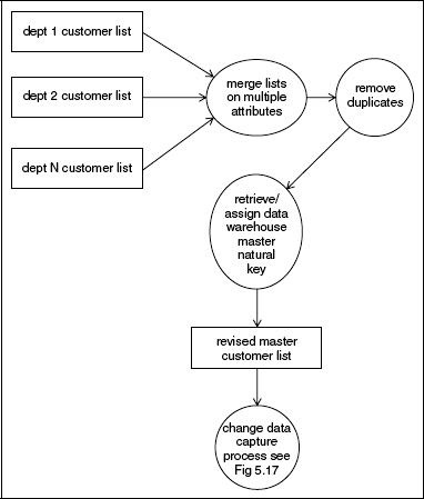
In the deduplication step, which is part of the data-cleaning module, each customer must be correctly identified across separate original data sources so that the total customer count is correct. A master natural key for the customer may have to be created by the data warehouse at this point. This would be a kind of enterprise-wide customer ID that would stay constant over time for any given customer.
In the conforming step, which is part of the data-conforming module, all attributes from the original sources that try to describe the same aspect of the customer need to be converted into single values used by all the departments. For example, a single set of address fields must be established for the customer. Finally, in the merge (survival) step, which is part of the delivery-module, all the remaining separate attributes from the individual source systems are unioned into one big, wide dimension record.
Later in this chapter, when we discuss slowly changing dimensions, we will see that the biggest dimensions are very sensitive to change, if it means that we generate new dimension records for each change. Hold that thought for a moment.
Small Dimensions
PROCESS CHECK Planning & Design:
Requirements/Realities → Architecture → Implementation → Test/Release
Data Flow: Extract → Clean → Conform → Deliver
Many of the dimensions in a data warehouse are tiny lookup tables with only a few records and one or two columns. For example, many transaction-grained fact tables have a transaction type dimension that provides labels for each kind of transaction. These tables are often built by typing into a spreadsheet and loading the data directly into the final physical dimension table. The original source spreadsheet should be kept because in many cases new records such as new transaction types could be introduced into the business.
Although a little dimension like transaction type may appear in many different data marts, this dimension cannot and should not be conformed across the various fact tables. Transaction types are unique to each production system.
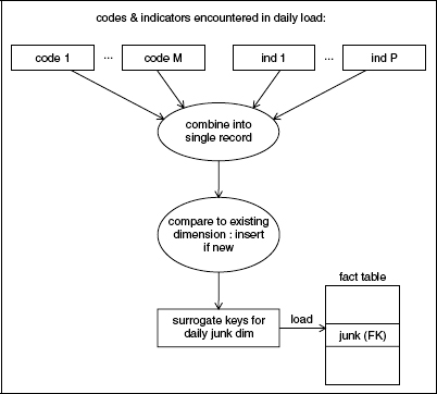
In some cases, little dimension tables that serve to decode operational values can be combined into a single larger dimension. This is strictly a tactical maneuver to reduce the number of foreign keys in a fact table. Some data sources have a dozen or more operational codes attached to fact table records, many of which have very low cardinalities. Even if there is no obvious correlation between the values of the operational codes, a single junk dimension can be created to bring all these little codes into one dimension and tidy up the design. The ETL data flow for a typical junk dimension is shown in Figure 5.7. The records in the junk dimension should probably be created as they are encountered in the data, rather than beforehand as the Cartesian product of all the separate codes. It is likely that the incrementally produced junk dimension is much smaller than the full Cartesian product of all the values of the codes. The next section extends this kind of junk-dimension reasoning to much larger examples, where the designer has to grapple with the problem of one dimension or two.
Figure 5.7 ETL data flow for a typical junk dimension.
One Dimension or Two
In dimensional modeling, we normally assume that dimensions are independent. In a strictly mathematical sense, this is almost never true. Although you may sell many products in many stores, the product dimension and the store dimension are probably not truly independent. Some products are sold in only selected stores. A good statistician would be able to demonstrate a degree of correlation between the product dimension and the store dimension. But such a finding normally does not deter us from creating separate product and store dimensions. The correlation that does exist between these dimensions can be faithfully and accurately depicted in the sales fact table.
Modeling the product dimension with the store dimension in this example would be a disaster. If you had a million-row product dimension and a 100-row store dimension, a combined dimension might approach 100 million rows! Bookkeeping the cross-correlations between dimensions solely in the fact table is an example of a powerful dimensional-modeling step: demoting the correlations between dimensions into a fact table.
A final nail in the coffin for combining product and store is that there may be more than one independent type of correlation between these two dimensions. We have discussed the merchandising correlation between these two dimensions, but there could be a pricing-strategy correlation, a warehousing correlation, or a changing-seasonality correlation. In general, tracking all of these complex relationships must be handled by leaving the dimensions simple and independent and by bookkeeping the cross-dimensional relationships in one or more fact tables.
At this point, you may be convinced that all dimensions can be independent and separate. But that’s because we have been discussing a somewhat extreme example of two big dimensions where the correlation is statistically weak. Are other situations not so black and white? First, let us immediately dispense with the completely correlated overlap of two dimensions. We should never have a single fact table with both a product dimension and a brand dimension if product rolls up to brand in a perfect many-to-1 relationship. In this case, product and brand are part of a hierarchy, and we should always combine these into a single dimension.
There are other cases where two candidate dimensions do not form a perfect hierarchy but are strongly correlated. To jump to the bottom line, if the correlation is reasonably high and the resulting combined dimension is reasonably small, the two dimensions should be combined into one. Otherwise, the dimensions should be left separate. The test for a reasonably high correlation should be made from the end user’s perspective. If the pattern of overlap between the two dimensions is interesting to end users and is constant and unchanging, the combined dimension may be attractive. Remember that the combined dimension in this case serves as an efficient target for queries, independent of any fact table. In our opinion, a dimension is no longer reasonably small when it becomes larger than 100,000 rows. Over time, perhaps technology will relax this arbitrary boundary, but in any case a 100,000 row dimension will always present some user-interface challenges!
Dimensional Roles
The data warehouse architect will frequently specify a dimension to be attached multiple times to the same fact table. These are called dimensional roles. Probably the most common role-playing dimension is the calendar date dimension. Many fact tables, especially the accumulating snapshot fact tables, have multiple date foreign keys. We discuss accumulating snapshot fact tables in Chapter 6. See Figure 5.8. Another common example of a role-playing dimension is the employee dimension, where different foreign keys in the fact table represent different types of employees being involved in a single transaction. See Figure 5.9.
In all role-playing dimension implementations, we recommend first building a generic single dimension table and then implementing each of the roles with a view on this generic table. See Figure 5.10. For instance, if we have an order-date, a shipment-date, a payment-date, and a return-date on an orders transaction accumulating snapshot fact table, we would first build a generic calendar date dimension and the create four views corresponding to the four dates needed. If the fields in each view are identically named, the application developer and possibly the end user will need to see the fully qualified names to distinguish similar fields from the different views in the same query. For that reason, we recommend creating distinguishable field names in the original view definitions so that every tool, even those not supported by metadata, will display the fields unambiguously.
Figure 5.8 A typical accumulating snapshot fact table.
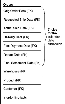
Figure 5.9 Two employee role playing dimensions.
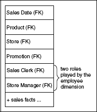
Figure 5.10 Multiple calendar role playing dimensions.

The recommended design of dimensional roles described previously makes the impact of dimensional roles on the ETL team equal to zero. So why do we discuss it? Our objective is to make sure the ETL team doesn’t generate multiple physical tables in cases where view definitions (roles) accomplish the same purpose.
Don’t use the dimensional-role techniques as an excuse to build abstract, super-large dimensions. For instance, in a telco environment, nearly everything has a location. If every possible location of every entity is represented in a single location dimension, this dimension could have millions of rows. Using a view on a multimillion row dimension in every application with a location dimension is probably a performance killer. In this case, actual physical dimensions created as extracted subsets of the big location dimension are probably better.
Dimensions as Subdimensions of Another Dimension
PROCESS CHECK Planning & Design:
Requirements/Realities → Architecture → Implementation → Test/Release
Data Flow: Extract → Clean → Conform → Deliver
Usually, we think of a reference to a dimension as a foreign key in a fact table. However, references to dimensions occasionally appear in other dimensions, and the proper foreign key should be stored in the parent dimension in the same way as a fact table. In other writings, we have sometimes referred to these subdimensions as outriggers. Let’s discuss two common examples.
Many dimensions have calendar dates embedded in them. Customer dimension records often have a first purchase date attribute. This should be modeled as a foreign key reference to the calendar date dimension, not as an SQL date stamp. See Figure 5.11. In this way, applications have access to all the extended calendar attributes when constraining on the first purchase date. This foreign key reference is really another kind of dimensional role played by the calendar date dimension. A separate view, in this case on the calendar date dimension, must be defined for each such reference.
Figure 5.11 Customer dimension showing two date treatments.
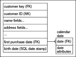
Note that not all dates stored in dimensions can be modeled as foreign key references to the calendar date dimension, since the calendar date dimension has a bounded duration. A customer’s birth date may well precede the first entry in the calendar date dimension. If that could happen, the customer birth date attribute must always be a simple SQL date stamp, not a foreign key reference. This is also shown in Figure 5.11.
A second common example of a dimension attached to a dimension is attaching an individual customer dimension to a bank account dimension. Although there might be many account holders in an account, usually a single customer is designated as the primary account holder. This primary account holder should be modeled as a foreign key reference in the account dimension to the customer dimension. See Figure 5.12.
Figure 5.12 A customer dimension used as a subdimension.

In this banking example, we have not handled the problem of many customers being associated with an account. We have dealt only with the single primary account holder customer. We will associate an open-ended number of customers to an account later in this chapter when we discuss multivalued dimensions and bridge tables.
To summarize this section, the ETL dimensional delivery module must convert selected fields in the input data for the dimension to foreign key references.
Degenerate Dimensions
PROCESS CHECK Planning & Design:
Requirements/Realities → Architecture → Implementation → Test/Release
Data Flow: Extract → Clean → Conform → Deliver
Whenever a parent-child data relationship is cast in a dimensional framework, the natural key of the parent is left over as an orphan in the design process. For example, if the grain of a fact table is the line item on an order, the dimensions of that fact table include all the dimensions of the line itself, as well as the dimensions of the surrounding order. Remember that we attach all single-valued dimensional entities to any given fact table record. When we have attached the customer and the order date and other dimensions to the design, we are left with the original order number. We insert the original order number directly into the fact table as if it were a dimension key. See Figure 5.13. We could have made a separate dimension out of this order number, but it would have turned out to contain only the order number, nothing else. For this reason, we give this natural key of the parent a special status and call it a degenerate (or empty) dimension. This situation arises in almost every parent-child design, including order numbers, shipment numbers, bill-of-lading numbers, ticket numbers, and policy numbers.
Figure 5.13 An order line accumulating snapshot fact table.
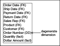
There is a danger that these source-system-generated numbers can get reused by different ERP instances installed in separate business units of an overall organization. For this reason, it may be a good idea to make a smart degenerate key value in these cases by prepending an organization ID onto the basic order number or sales ticket number.
Slowly Changing Dimensions
PROCESS CHECK Planning & Design:
Requirements/Realities → Architecture → Implementation → Test/Release
Data Flow: Extract → Clean → Conform → Deliver
When the data warehouse receives notification that an existing row in a dimension has in some way changed, there are three basic responses. We call these three basic responses Type 1, Type 2, and Type 3 slowly changing dimensions (SCDs).
Type 1 Slowly Changing Dimension (Overwrite)
The Type 1 SCD is a simple overwrite of one or more attributes in an existing dimension record. See Figure 5.14. The ETL processing would choose the Type 1 approach if data is being corrected or if there is no interest in keeping the history of the previous values and no need to run prior reports. The Type 1 overwrite is always an UPDATE to the underlying data, and this overwrite must be propagated forward from the earliest permanently stored staging tables in the ETL environment so that if any of them are used to recreate the final load tables, the effect of the overwrite is preserved. This point is expanded in Chapter 8.
Figure 5.14 Processing a Type 1 SCD.
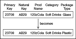
Although inserting new records into a Type 1 SCD requires the generation of new dimension keys, processing changes in a Type 1 SCD never affects dimension table keys or fact table keys and in general has the smallest impact on the data of the three SCD types. The Type 1 SCD can have an effect on the storage of aggregate fact tables, if any aggregate is built directly on the attribute that was changed. This issue will be described in more detail in Chapter 6.
Some ETL tools contain UPDATE else INSERT functionality. This functionality may be convenient for the developer but is a performance killer. For maximum performance, existing records (UPDATEs) should be segregated from new ones (INSERTs) during the ETL process; each should be fed to the data warehouse independently. In a Type 1 environment, you may not know whether an incoming record is an UPDATE or an INSERT. Some developers distinguish between a VERY SCD (very slowly changing dimension) where INSERTs predominate and a Fastly Changing Dimension (FCD?). They use INSERT else UPDATE logic for VERY SCDs and UPDATE else INSERT logic for the FCDs. We hope this terminology doesn’t catch on.
In most data warehouse implementations, the size of the majority of dimensions is insignificant. When you are loading small tables that do not warrant the complexity of invoking a bulk loader, Type 1 changes can be applied via normal SQL DML statements. Based on the natural key extracted from the source system, any new record is assigned a new surrogate key and appended to the existing dimension data. Existing records are updated in place. Performance of this technique may be poorer as compared with being loaded via a bulk loader, but if the tables are of reasonable size, the impact should be negligible.
Some ETL tools offer specialized transformations that can detect whether a record needs to be inserted or updated. However, this utility must ping the table using the primary key of the candidate record to see if it exists. This approach is process intensive and should be avoided. To minimize the performance hit when using SQL to load a Type 1 dimension, the ETL process should explicitly segregate existing data that requires UPDATE statements from data that requires INSERT.
Type 1 SCD changes can cause performance problems in ETL processing. If this technique is implemented using SQL data-manipulation language (DML), most database management systems will log the event, hindering performance.
A database log is implicitly created and maintained by the DBMS. Database logging is constructive for transaction processing where data is entered by many users in an uncontrolled fashion. Uncontrolled is used because in the on-line transaction processing (OLTP) environment, there is no way to control unpredicted user behavior, such as closing a window midway through an update. The DBMS may need to ROLLBACK, or undo, a failed update. The database log enables this capability.
Conversely, in the data warehouse, all data loading is controlled by the ETL process. If the process fails, the ETL process should have the capability to recover and pick-up where it left off, making the database log superfluous.
With database logging enabled, large dimensions will load at an unacceptable rate. Some database management systems allow you to turn logging off during certain DML processes, while others require their bulk loader to be invoked for data to be loaded without logging.
Bulk Loading Type 1 Dimension Changes
Because Type 1 overwrites data, the easiest implementation technique is to use SQL UPDATE statements to make all of the dimension attributes correctly reflect the current values. Unfortunately, as a result of database logging, SQL UPDATE is a poor-performing transaction and can inflate the ETL load window. For very large Type 1 changes, the best way to reduce DBMS overhead is to employ its bulk loader. Prepare the new dimension records in a separate table. Then drop the records from the dimension table and reload them with the bulk loader.
Type 2 Slowly Changing Dimension (Partitioning History)
The Type 2 SCD is the standard basic technique for accurately tracking changes in dimensional entities and associating them correctly with fact tables. The basic idea is very simple. When the data warehouse is notified that an existing dimension record needs to be changed, rather than overwriting, the data warehouse issues a new dimension record at the moment of the change. This new dimension record is assigned a fresh surrogate primary key, and that key is used from that moment forward in all fact tables that have that dimension as a foreign key. As long as the new surrogate key is assigned promptly at the moment of the change, no existing keys in any fact tables need to be updated or changed, and no aggregate fact tables need to be recomputed. The more complex case of handling late-arriving notifications of changes is described later in this chapter.
We say that the Type 2 SCD perfectly partitions history because each detailed version of a dimensional entity is correctly connected to the span of fact table records for which that version is exactly correct. In Figure 5.15, we illustrate this concept with a slowly changing employee dimension where a particular employee named Jane Doe is first a trainee, then a regular employee, and finally a manager. Jane Doe’s natural key is her employee number and that remains constant throughout her employment. In fact, the natural key field always has the unique business rule that it cannot change, whereas every other attribute in the employee record can change. Jane Doe’s primary surrogate key takes on three different values as she is promoted, and these surrogate primary keys are always correctly associated with contemporary fact table records. Thus, if we constrain merely on the employee Jane Doe, perhaps using her employee number, we pick up her entire history in the fact table because the database picks up all three surrogate primary keys from the dimension table and joins them all to the fact table. But if we constrain on Jane Doe, manager, we get only one surrogate primary key and we see only the portion of the fact table for which Jane Doe was a manager.
Figure 5.15 The Type 2 SCD perfectly partitions history.

If the natural key of a dimension can change, from the data warehouse’s point of view, it isn’t really a natural key. This might happen in a credit card processing environment where the natural key is chosen as the card number. We all know that the card number can change; thus, the data warehouse is required to use a more fundamental natural key. In this example, one possibility is to use the original customer’s card number forever as the natural key, even if it subsequently changes. In such a design, the customer’s current contemporary card number would be a separate field and would not be designated as a key.
The Type 2 SCD requires a good change data capture system in the ETL environment. Changes in the underlying source data need to be detected as soon as they occur, so that a new dimension record in the data warehouse can be created. We discuss many of the issues of change data capture at extract time in Chapter 3. In the worst scenario, the underlying source system does not notify the data warehouse of changes and does not date-stamp its own updates. In this case, the data warehouse is forced to download the complete dimension and look record by record and field by field for changes that have occurred since the last time the dimension was downloaded from the source. Note that this requires the prior extract (the master dimension cross reference file) from the dimension’s source to be explicitly staged in the ETL system. See Figure 5.16.
Figure 5.16 Dimension table surrogate key management.
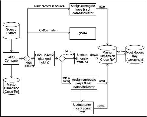
For a small dimension of a few thousand records and a dozen fields, such as a simple product file, the detection of changes shown in Figure 5.16 can be done by brute force, comparing every field in every record in today’s download with every field in every record from yesterday. Additions, changes, and deletions need to be detected. But for a large dimension, such as a list of ten million insured health care patients with 100 descriptive fields in each record, the brute-force approach of comparing every field in every record is too inefficient. In these cases, a special code known as a CRC is computed and associated with every record in yesterday’s data. The CRC (cyclic redundancy checksum) code is a long integer of perhaps 20 digits that is exquisitely sensitive to the information content of each record. If only a single character in a record is changed, the CRC code for that record will be completely different. This allows us to make the change data capture step much more efficient. We merely compute the CRC code for each incoming new record by treating the entire record as a single text string, and we compare that CRC code with yesterday’s code for the same natural key. If the CRCs are the same, we immediately skip to the next record. If the CRCs are different, we must stop and compare each field to find what changed. The use of this CRC technique can speed up the change data capture process by a factor of 10. At the time of this writing, CRC calculation modules are available from all of the leading ETL package vendors, and the code for implementing a CRC comparison can be readily found in textbooks and on the Internet.
Once a changed dimension record has been positively identified, the decision of which SCD type is appropriate can be implemented. Usually, the ETL system maintains a policy for each column in a dimension that determines whether a change in that attribute triggers a Type 1, 2, or 3 response, as shown in Figure 5.16.
To identify records deleted from the source system, you can either read the source transaction log file (if it is available) or note that the CRC comparison step described previously cannot find a record to match a natural key in the ETL system’s comparison file. But in either case, an explicit business rule must be invoked to deal with the deletion. In many cases, the deleted entity (such as a customer) will have a continuing presence in the data warehouse because the deleted entity was valid in the past. If the business rule conclusively states that the deleted entity can no longer appear in subsequent loads from the dimension-table source, the deleted entity can be removed from the daily comparison step, even though in the historical dimension tables and fact tables it will live on.
Without transaction log files, checking for deleted data is a process- intensive practice and usually is implemented only when it is demanded. An option that has proven to be effective is utilizing the MINUS set operator to compare the natural keys from the dimension in the data warehouse against the natural keys in the source system table. UNION and MINUS are SET operators supported by most database management systems used to compare two sets of data. These operators are extremely powerful for evaluating changes between the source and target. However, for these SET operators to work, the two tables need to be in the same database, or a database link must be created. Some ETL tools support SET operations between heterogeneous systems. If this is a critical requirement for your environment, be sure it is included in your proof-of-concept criteria when selecting your ETL toolset.
Notice in Figure 5.16 that when we have created the new surrogate key for a changed dimension entity, we update a two-column lookup table, known as the most recent key lookup table for that dimension. These little tables are of immense importance when loading fact table data. Hold this thought until you read the surrogate key pipeline section in Chapter 6.
The same benefits that the lookup-table solution offers can be accomplished by storing all of the relevant natural keys directly in the dimension table. This approach is probably the most common for determining whether natural keys and dimension records have been loaded. This approach makes the associated natural keys available to the users, right in the dimension. The major benefit of this strategy over the lookup table is that the surrogate key exists only in one place, eliminating the risk of the dimension and the mapping table becoming out of sync. During the ETL, the process selects the natural key from the appropriate column within the dimension where it equals the incoming natural key. If a match is found, the process can apply any of the SCD strategies described later in this chapter.
If the key is not found, it can generate a surrogate key using any of the methods discussed in the next section and insert a new record.
Looking directly to dimensions is favored by many data warehouse designers because it exposes the data lineage to users. By having the natural keys directly in the dimension, users know exactly where the data in the dimension came from and can verify it in the source system. Moreover, natural keys in the dimension relieve the ETL and DBA teams from having to maintain a separate mapping table for this purpose. Finally, this approach makes a lot of sense in environments where there is a large fraction of late-arriving data where the most recent advantages of a lookup table cannot be used.
In this section, we have described a change-data-capture scenario in which the data warehouse is left to guess if a change occurred in a dimension record and why. Obviously, it would be preferable if the source system handed over only the changed records (thereby avoiding the complex comparison procedure described previously) and ideally accompanied the changed records with reason codes that distinguished the three SCD responses. What a lovely dream.
Our approach allows us to respond to changes in the source for a dimension as they occur, even when the changes are not marked. A more difficult situation takes place when a database is being loaded for the first time from such an uncooperative source. In this case, if the dimension has been overwritten at the source, it may be difficult to reconstruct the historical changes that were processed unless original transaction log files are still available.
Precise Time Stamping of a Type 2 Slowly Changing Dimension
The discussion in the previous section requires only that the ETL system generate a new dimension record when a change to an existing record is detected. The new dimension record is correctly associated with fact table records automatically because the new surrogate key is used promptly in all fact table loads after the change takes place. No date stamps in the dimension are necessary to make this correspondence work.
Having said that, it is desirable in many situations to instrument the dimension table to provide optional useful information about Type 2 changes. We recommend adding the following five fields to dimension tables processed with Type 2 logic:
Calendar Date foreign key (date of change)
Row Effective DateTime (exact date-time of change)
Row End DateTime (exact date-time of next change)
Reason for Change (text field)
Current Flag (current/expired)
These five fields make the dimension a powerful query target by itself, even if no fact table is mentioned in the query. The calendar date foreign key allows an end user to use the business calendar (with seasons, holidays, paydays, and fiscal periods) to ask how many changes of a particular type were made in certain business-significant periods. For instance, if the dimension is a human resources employee table, one could ask how many promotions occurred in the last fiscal period.
The two SQL date-time stamps define an exact interval in which the current dimension record correctly and completely describes the entity. When a new change is processed, the Row Effective DateTime is set to the current date and time, and the Row End DateTime is set to an arbitrary time far in the future. When a subsequent change to this dimension entity is processed, the previous record must be revisited and the Row End DateTime set to the proper value. If this procedure is followed, the two date-time stamps always define an interval of relevance so that queries can specify a random specific date and time and use the SQL BETWEEN logic to immediately deliver records that were valid at that instant. We need to set the Row End DateTime to a real value, even when the record is the most current, so that the BETWEEN logic doesn’t return an error if the second date is represented as null.
It is seems to be universal practice for back-end scripts to be run within the transaction database to modify data without updating respective metadata fields, such as the last_modified_date. Using these fields for the dimension row effective_datetime will cause inconsistent results in the data warehouse. Do not depend on metadata fields in the transaction system. Always use the system or as of date to derive the row effective_datetime in a Type 2 slowly changing dimension.
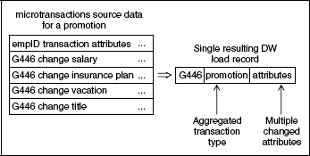
The Reason for Change field probably needs to come from the original data-entry process that gave rise to the changed dimension record. For instance, in the human resources example, you would like a promotion to be represented as a single new record, appropriately time stamped, in the employee dimension. The Reason for Change field should say promotion. This may not be as easy as it sounds. The HR system may deliver a number of change records at the time of an employee’s promotion if several different employee attributes (job grade, vacation benefits, title, organization and so on) change simultaneously. The challenge for the data warehouse is to coalesce these changes into a single new dimension record and correctly label this new record with promotion. Such a coalescing of underlying transaction records into a kind of aggregated super-transaction may be necessary with some source systems, even if no attempt is made to ascribe a reason code to the overall change. We have seen relatively simple updates such as employee promotions represented by dozens of micro transactions. The data warehouse should not carry these microtransactions all the way to the final end user tables, because the individual microtransactions may not have real business significance. This processing is depicted in Figure 5.17. Finally, the Current Flag is simply a convenient way to retrieve all the most-current records in a dimension. It is indeed redundant with the two SQL date-time stamps and therefore can be left out of the design. This flag needs to be set to EXPIRED when a superceding change to the dimension entity takes place.
Figure 5.17 Consolidating source system microtransactions.
Type 3 Slowly Changing Dimension (Alternate Realities)
The Type 3 SCD is used when a change happens to a dimension record but the old value of the attribute remains valid as a second choice. The two most common business situations where this occurs are changes in sales-territory assignments, where the old territory assignment must continue to be available as a second choice, and changes in product-category designations, where the old category designation must continue to be available as a second choice. The data warehouse architect should identify fields that require Type 3 administration.
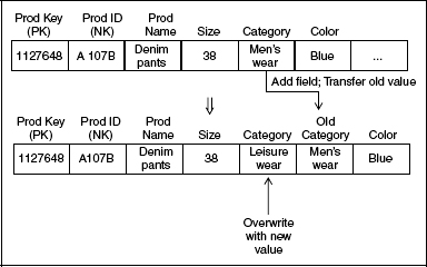
In a Type 3 SCD, instead of issuing a new row when a change takes place, a new column is created (if it does not already exist), and the old value is placed in this new field before the primary value is overwritten. For the example of the product category, we assume the main field is named Category. To implement the Type 3 SCD, we alter the dimension table to add the field Old Category. At the time of the change, we take the original value of Category and write it into the Old Category field; then we overwrite the Category field as if it were a Type 1 change. See Figure 5.18. No keys need to be changed in any dimension table or in any fact table. Like the Type 1 SCD, if aggregate tables have been built directly on the field undergoing the Type 3 change, these aggregate tables need to be recomputed. This procedure is described in Chapter 6.
Figure 5.18 Implementing the Type 3 SCD for a product-category description.
Type 3 changes often do not come down the normal data-flow pipeline. Rather, they are executive decisions communicated to the ETL team, often verbally. The product-category manager says, “Please move Brand X from Mens Sportswear to Leather Goods, but let me track Brand X optionally in the old category.” The Type 3 administration is then kicked off by hand, and can even involve a schema change, if the changed attribute (in this case, brand) does not have an alternate field.
When a new record is added to a dimension that contains Type 3 fields, a business rule must be invoked to decide how to populate the old value field. The current value could be written into this field, or it could be NULL, depending on the business rule.
We often describe the Type 3 SCD as supporting an alternate reality. In our product-category example, the end user could choose between two versions of the mapping of products to categories.
The Type 3 SCD approach can be extended to many alternate realities by creating an arbitrary number of alternate fields based on the original attribute. Occasionally, such a design is justified when the end user community already has a clear vision of the various interpretations of reality. Perhaps the product categories are regularly reassigned but the users need the flexibility to interpret any span of time with any of the category interpretations. The real justification for this somewhat awkward design is that the user interface to this information falls out of every query tool with no programming, and the underlying SQL requires no unusual logic or extra joins. These advantages trump the objections to the design using positionally dependent attributes (the alternate fields).
Hybrid Slowly Changing Dimensions
The decision to respond to changes in dimension attributes with the three SCD types is made on a field-by-field basis. It is common to have a dimension containing both Type 1 and Type 2 fields. When a Type 1 field changes, the field is overwritten. When a Type 2 field changes, a new record is generated. In this case, the Type 1 change needs to be made to all copies of the record possessing the same natural key. In other words, if the ethnicity attribute of an employee profile is treated as a Type 1, if it is ever changed (perhaps to correct an original erroneous value), the ethnicity attribute must be overwritten in all the copies of that employee profile that may have been spawned by Type 2 changes.
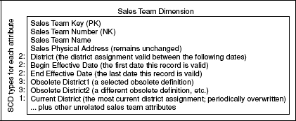
It is possible to combine all the SCD types in a single dimension record. See Figure 5.19. In this example, the district assignment field for the sales team is a Type 2 attribute. Whenever the district assignment changes, a new record is created, and the beginning and effective dates are set appropriately. The set of yearly old district assignments are Type 3 fields, implementing many alternate realities. And finally, the current district assignment is a Type 1 field, and it is overwritten in all copies of the sales team dimension records whenever the current district is reassigned.
Figure 5.19 A hybrid SCD showing all three types.
Late-Arriving Dimension Records and Correcting Bad Data
PROCESS CHECK Planning & Design:
Requirements/Realities → Architecture → Implementation → Test/Release
Data Flow: Extract → Clean → Conform → Deliver
Late-arriving data may need to be extracted via a different application or different constraints compared to normal contemporary data. Bad data obviously is picked up in the data-cleaning step.
A late-arriving dimension record presents a complex set of issues for the data warehouse. Suppose that we have a fictitious product called Zippy Cola. In the product dimension record for Zippy Cola 12-ounce cans, there is a formulation field that has always contained the value Formula A. We have a number of records for Zippy Cola 12-ounce cans because this is a Type 2 slowly changing dimension and other attributes like the package type and the subcategory for Zippy Cola 12-ounce cans have changed over the past year or two.
Today we are notified that on July 15, 2003 (a year ago) the formulation of Zippy Cola 12-ounce cans was changed to Formula B and has been Formula B ever since. We should have processed this change a year ago, but we failed to do so. Fixing the information in the data warehouse requires the following steps:
1. Insert a fresh new record with a new surrogate key for Zippy Cola 12-ounce cans into the Product dimension with the formulation field set to Formula B, the row effective datetime set to July 15, 2003, and the row end datetime set to the row effective datetime of the next record for Zippy Cola in the product dimension table. We also need to find the closest previous dimension record for Zippy Cola and set its row end datetime to the datetime of our newly inserted record. Whew!
2. Scan forward in the Product dimension table from July 15, 2003, finding any other records for Zippy Cola 12-ounce cans, and destructively overwrite the formulation field to Formula B in all such records.
3. Find all fact records involving Zippy Cola 12-ounce cans from July 15, 2003, to the first next change for that product in the dimension after July 15, 2003, and destructively change the Product foreign key in those fact records to be the new surrogate key created in Step 1.
Updating fact table records (in Step 3) is a serious step that should be tested carefully in a test environment before performing it on the production system. Also, if the update is protected by a database transaction, be careful that some of your updates don’t involve an astronomical number of records. For operational purposes, such large updates should be divided into chunks so that you don’t waste time waiting for an interrupted update of a million records to roll back.
There are some subtle issues here. First, we need to check to see if some other change took place for Zippy Cola 12-ounce cans on July 15, 2003. If so, we need only to perform Step 2. We don’t need a new dimension record in this special case.
In general, correcting bad data in the data warehouse can involve the same logic. Correcting a Type 1 field in a dimension is simplest because we just have to overwrite all instances of that field in all the records with the desired natural key. Of course, aggregate tables have to be recalculated if they have specifically been built on the affected attribute. Please see the aggregate updating section for fact tables in Chapter 6. Correcting a Type 2 field requires thoughtful consideration, since it is possible that the incorrect value has a specific time span.
This discussion of late-arriving dimension records is really about late-arriving versions of dimension records. In real-time systems (discussed in Chapter 11), we deal with true late-arriving dimension records that arrive after fact records have already been loaded into the data warehouse. In this case, the surrogate key in the fact table must point to a special temporary placeholder in the dimension until the real dimension record shows up.
Multivalued Dimensions and Bridge Tables
PROCESS CHECK Planning & Design:
Requirements/Realities → Architecture → Implementation → Test/Release
Data Flow: Extract → Clean → Conform → Deliver
Occasionally a fact table must support a dimension that takes on multiple values at the lowest level of granularity of the fact table. Examples described in the other Toolkit books include multiple diagnoses at the time of a billable health care treatment and multiple account holders at the time of a single transaction against a bank account.
If the grain of the fact table is not changed, a multivalued dimension must be linked to the fact table through an associative entity called a bridge table. See Figure 5.20 for the health care example.
Figure 5.20 Using a bridge table to represent multiple diagnoses.

To avoid a many-to-many join between the bridge table and the fact table, one must create a group entity related to the multivalued dimension. In the health care example, since the multivalued dimension is diagnosis, the group entity is diagnosis group. The diagnosis group becomes the actual normal dimension to the fact table, and the bridge table keeps track of the many-to-many relationship between diagnosis groups and diagnoses. In the bank account example, when an account activity record is linked to the multivalued customer dimension (because an account can have many customers), the group entity is the familiar account dimension.
The challenge for the ETL team is building and maintaining the group entity table. In the health care example, as patient-treatment records are presented to the system, the ETL system has the choice of either making each patient’s set of diagnoses a unique diagnosis group or reusing diagnosis groups when an identical set of diagnoses reoccurs. There is no simple answer for this choice. In an outpatient setting, diagnosis groups would be simple, and many of the same ones would appear with different patients. In this case, reusing the diagnosis groups is probably the best choice. See Figure 5.21. But in a hospital environment, the diagnosis groups are far more complex and may even be explicitly time varying. In this case, the diagnosis groups should probably be unique for each patient and each hospitalization. See Figure 5.22 and the discussion of time-varying bridge tables that follows. The admission and discharge flags are convenient attributes that allow the diagnosis profiles at the time of admission and discharge to be easily isolated.
Figure 5.21 Processing diagnosis groups in an outpatient setting.
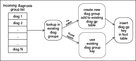
Figure 5.22 A time-varying diagnosis group bridge table appropriate for a hospital setting.

Administering the Weighting Factors
The diagnosis group tables illustrated in Figures 5.20 and 5.22 include weighting factors that explicitly prorate the additive fact (charge dollars) by each diagnosis. When a requesting query tool constrains on one or more diagnoses, the tool can chose to multiply the weighting factor in the bridge table to the additive fact, thereby producing a correctly weighted report. A query without the weighting factor is referred to as an impact report. We see that the weighting factor is nothing more than an explicit allocation that must be provided in the ETL system. These allocations are either explicitly fetched from an outside source like all other data or can be simple computed fractions depending on the number of diagnoses in the diagnosis group. In the latter case, if there are three diagnoses in the group, the weighting factor is 1/3 = 0.333 for each diagnosis.
In many cases, a bridge table is desirable, but there is no rational basis for assigning weighting factors. This is perfectly acceptable. The user community in this case cannot expect to produce correctly weighted reports. These front-room issues are explored in some depth in the Data Warehouse Toolkit, Second Edition in the discussion of modeling complex events like car accidents.
Time-Varying Bridge Tables
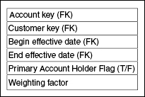
If the multivalued dimension is a Type 2 SCD, the bridge table must also be time varying. See Figure 5.23 using the banking example. If the bridge table were not time varying, it would have to use the natural keys of the customer dimension and the account dimension. Such a bridge table would potentially misrepresent the relationship between the accounts and customers. It is not clear how to administer such a table with natural keys if customers are added to or deleted from an account. For these reasons, the bridge table must always contain surrogate keys. The bridge table in Figure 5.23 is quite sensitive to changes in the relationships between accounts and customers. New records for a given account with new begin-date stamps and end-date stamps must be added to the bridge table whenever:
Figure 5.23 A time-varying bridge table for accounts and customers.
The account record undergoes a Type 2 update
Any constituent customer record undergoes a Type 2 update
A customer is added to or deleted from the account or
The weighting factors are adjusted
Ragged Hierarchies and Bridge Tables
PROCESS CHECK Planning & Design:
Requirements/Realities → Architecture → Implementation → Test/Release
Data Flow: Extract → Clean → Conform → Deliver
Ragged hierarchies of indeterminate depth are an important topic in the data warehouse. Organization hierarchies such as depicted in Figure 5.24 are a prime example. A typical organization hierarchy is unbalanced and has no limits or rules on how deep it might be.
There are two main approaches to modeling a ragged hierarchy, and both have their pluses and minuses. We’ll discuss these tradeoffs in terms of the customer hierarchy shown in Figure 5.24.
Figure 5.24 A representative ragged organization hierarchy.

The recursive pointer approach shown in Figure 5.25.
Figure 5.25 A customer dimension with a recursive pointer.
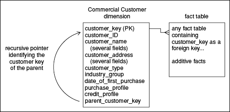
(+) embeds the hierarchy relationships entirely in the customer dimension
(+) has simple administration for adding and moving portions of the hierarchy
but
(-) requires nonstandard SQL extensions for querying and may exhibit poor query performance when the dimension is joined to a large fact table
(-) can only represent simple trees where a customer can have only one parent (that is, disallowing shared ownership models)
(-) cannot support switching between different hierarchies
(-) is very sensitive to time-varying hierarchies because the entire customer dimension undergoes Type 2 changes when the hierarchy is changed
The hierarchy bridge table approach shown in Figure 5.26:
Figure 5.26 A hierarchy bridge table representing customer ownership.
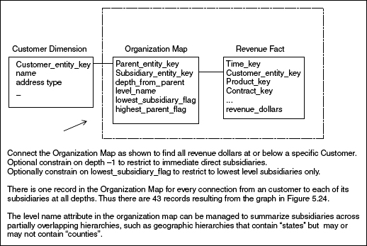
(+) isolates the hierarchy relationships in the bridge table, leaving the customer dimension unaffected
(+) is queried with standard SQL syntax using single queries that evaluate the whole hierarchy or designated portions of the hierarchy such as just the leaf nodes
(+) can be readily generalized to handle complex trees with shared ownership and repeating subassemblies
(+) allows instant switching between different hierarchies because the hierarchy information is entirely concentrated in the bridge table and the bridge table is chosen at query time
(+) can be readily generalized to handle time-varying Type 2 ragged hierarchies without affecting the primary customer dimension
but
(-) requires the generation of a separate record for each parent-child relationship in the tree, including second-level parents, third-level parents, and so on. Although the exact number of records is dependent on the structure of the tree, a rough rule of thumb is three times the number of records as nodes in the tree. Forty-three records are required in the bridge table to support the tree shown in Figure 5.24.
(-) involves more complex logic than the recursive pointer approach in order to add and move structure within the tree
(-) requires updating the bridge table when Type 2 changes take place within the customer dimension
Technical Note: POPULATING HIERARCHY BRIDGE TABLES
In February 2001, the following technical note on building bridge tables for ragged hierarchies was published as one of Ralph Kimball’s monthly design tips. Because it is so relevant to the ETL processes covered in this book, we reproduce it here, edited slightly, to align the vocabulary precisely with the book.
This month’s tip follows on from Ralph’s September 1998 article “Help for Hierarchies” (www.dbmsmag.com/9809d5.html), which addresses hierarchical structures of variable depth which are traditionally represented in relational databases as recursive relationships. Following is the usual definition of a simple company dimension that contains such a recursive relationship between the foreign key PARENT_KEY and primary key COMPANY_KEY.
Create table COMPANY (
COMPANY_KEY INTEGER NOT NULL,
COMPANY_NAME VARCHAR2(50),
(plus other descriptive attributes… ),
PARENT_KEY INTEGER);
While this is efficient for storing information on organizational structures, it is not possible to navigate or rollup facts within these hierarchies using the nonprocedural SQL that can be generated by commercial query tools. Ralph’s original article describes a bridge table similar to the one that follows that contains one record for each separate path from each company in the organization tree to itself and to every subsidiary below it that solves this problem.
Create table COMPANY_STRUCTURE (
PARENT_KEY INTEGER NOT NULL,
SUBSIDIARY_KEY INTEGER NOT NULL,
SUBSIDIARY_LEVEL INTEGER NOT NULL,
SEQUENCE_NUMBER INTEGER NOT NULL,
LOWEST_FLAG CHAR(1),
HIGHEST_FLAG CHAR(1),
PARENT_COMPANY VARCHAR2(50),
SUBSIDIARY_COMPANY VARCHAR2(50));
The last two columns in this example, which denormalize the company names into this table, are not strictly necessary but have been added to make it easy to see what’s going on later.
The following PL/SQL stored procedure demonstrates one possible technique for populating this hierarchy explosion bridge table from the COMPANY table on Oracle:
CREATE or Replace procedure COMPANY_EXPLOSION_SP as CURSOR Get_Roots is select COMPANY_KEY ROOT_KEY,
decode(PARENT_KEY, NULL,’Y’,’N’) HIGHEST_FLAG,
COMPANY_NAME ROOT_COMPANY
from COMPANY;
BEGIN
For Roots in Get_Roots
LOOP
insert into COMPANY_STRUCTURE
(PARENT_KEY,
SUBSIDIARY_KEY,
SUBSIDIARY_LEVEL,
SEQUENCE_NUMBER,
LOWEST_FLAG,
HIGHEST_FLAG,
PARENT_COMPANY,
SUBSIDIARY_COMPANY)
select
roots.ROOT_KEY,
COMPANY_KEY,
LEVEL - 1,
ROWNUM,
’N’,
roots.HIGHEST_FLAG,
roots.ROOT_COMPANY,
COMPANY_NAME
from
COMPANY
Start with COMPANY_KEY = roots.ROOT_KEY
connect by prior COMPANY_KEY = PARENT_KEY;
END LOOP;
update COMPANY_STRUCTURE
SET LOWEST_FLAG = ’Y’
where not exists (select * from COMPANY
where PARENT_KEY = COMPANY_STRUCTURE.SUBSIDIARY_KEY);
COMMIT;
END; /* of procedure */
This solution takes advantage of Oracle’s CONNECT BY SQL extension to walk each tree in the data while building the bridge table. While CONNECT BY is very useful within this procedure, it could not be used by an ad-hoc query tool for general-purpose querying. If the tool can generate this syntax to explore the recursive relationship, it cannot in the same statement join to a fact table. Even if Oracle were to remove this somewhat arbitrary limitation, the performance at query time would probably not be too good.
The following fictional company data will help you understand the COMPANY_STRUCTURE table and COMPANY_EXPLOSION_SP procedure:
/* column order is Company_key,Company_name,Parent_key */
insert into company values (100,’Microsoft’,NULL);
insert into company values (101,’Software’,100);
insert into company values (102,’Consulting’,101);
insert into company values (103,’Products’,101);
insert into company values (104,’Office’,103);
insert into company values (105,’Visio’,104);
insert into company values (106,’Visio Europe’,105);
insert into company values (107,’Back Office’,103);
insert into company values (108,’SQL Server’,107);
insert into company values (109,’OLAP Services’,108);
insert into company values (110,’DTS’,108);
insert into company values (111,’Repository’,108);
insert into company values (112,’Developer Tools’,103);
insert into company values (113,’Windows’,103);
insert into company values (114,’Entertainment’,103);
insert into company values (115,’Games’,114);
insert into company values (116,’Multimedia’,114);
insert into company values (117,’Education’,101);
insert into company values (118,’Online Services’,100);
insert into company values (119,’WebTV’,118);
insert into company values (120,’MSN’,118);
insert into company values (121,’MSN.co.uk’,120);
insert into company values (122,‘Hotmail.com’,120);
insert into company values (123,‘MSNBC’,120);
insert into company values (124,‘MSNBC Online’,123);
insert into company values (125,‘Expedia’,120);
insert into company values (126,‘Expedia.co.uk’,125);
/* End example data */
The procedure will take the 27 COMPANY records and create 110 COMPANY_STRUCTURE records make up of one big tree (Microsoft) with 27 nodes and 26 smaller trees. For large datasets, you may find that performance can be enhanced by adding a pair of concatenated indexes on the CONNECT BY columns. In this example, you could build one index on COMPANY_KEY,PARENT_KEY and the other on PARENT_KEY, COMPANY_KEY.
If you want to visualize the tree structure textually, the following query displays an indented subsidiary list for Microsoft:
select LPAD( ’ ’, 3*(SUBSIDIARY_LEVEL)) || SUBSIDIARY_COMPANY from COMPANY_STRUCTURE order by SEQUENCE_NUMBER
where PARENT_KEY = 100.
The SEQUENCE_NUMBER has been added since Ralph’s original article; it numbers nodes top to bottom, left to right. It allows the correct level-2 nodes to be sorted below their matching level-1 nodes.
For a graphical version of the organization tree, take a look at Visio 2000 Enterprise Edition, which has a database or text-file-driven organization chart wizard. With the help of VBA script, a view on the COMPANY_STRUCTURE table, and a fact table, it might automate the generation of just the HTML pages you want.
Using Positional Attributes in a Dimension to Represent Text Facts
The SQL interface to relational databases places some severe restrictions on certain kinds of analyses that need to perform complex comparisons across dimension records. Consider the following example of a text fact.
Suppose that we measure numeric values for recency, frequency, and intensity (RFI) of all our customers. We call in our data-mining colleagues and ask them to identify the natural clusters of customers in this abstract cube labeled by recency, frequency, and intensity. We really don’t want all the numeric results; we want behavioral clusters that are meaningful to our marketing department. After running the cluster identifier data-mining step, we find, for example, eight natural clusters of customers. After studying where the centroids of the clusters are located in our RFI cube, we are able to assign behavior descriptions to the eight behavior clusters:
A: High-volume repeat customer, good credit, few product returns
B: High-volume repeat customer, good credit, but many product returns
C: Recent new customer, no established credit pattern
D: Occasional customer, good credit
E: Occasional customer, poor credit
F: Former good customer, not seen recently
G: Frequent window shopper, mostly unproductive
H: Other
We can view the tags A through H as text facts summarizing a customer’s behavior. There aren’t a lot of text facts in data warehousing, but these behavior tags seem to be pretty good examples. We can imagine developing a time series of behavior-tag measurements for a customer over time with a data point each month:
John Doe: C C C D D A A A B B
This little time series is pretty revealing. How can we structure our data warehouse to pump out these kinds of reports? And how can we pose interesting constraints on customers to see only those who have gone from cluster A to cluster B in the most recent time period? We require even more complex queries such as finding customers who were an A in the 5th, 4th, or 3rd previous time period and are a B or a C in either the 2nd or 1st previous period.
We can model this time series of textual behavior tags in several different ways. Each approach has identical information content but differs significantly in ease of use. Let’s assume we generate a new behavior tag for each customer each month. Here are three approaches:
1. Fact table record for each customer for each month, with the behavior tag as a textual fact
2. Slowly changing customer dimension record (Type 2) with the behavior tag as a single attribute (field). A new customer record is created for each customer each month. Same number of new records each month as choice #1.
3. Single customer dimension record with a 24 month time series of behavior tags as 24 attributes, a variant of the Type 3 SCD many alternate realities approach
The whole point of this section is that choices 1 and 2, which create separate records for each behavior tag, leave the data warehouse with a structure that is effectively impossible to query. SQL has no direct approach for posing constraints across records. A sufficiently clever programmer can, of course, do anything, but each complex constraint would need to be programmed by hand. No standard query tool can effectively address design choices 1 or 2.
Design choice 3, shown in Figure 5.27, elegantly solves the query problem. Standard query tools can issue extremely complex straddle constraints against this design involving as many of the behavior tags as the user needs, because all the targets of the constraints are in the same record. Additionally, the resulting dimension table can be efficiently indexed with bitmap indexes on each of the low-cardinality behavior tags, so that performance can be excellent, even for complex queries.
Figure 5.27 Using positional attributes to model text facts.

There are several ways to maintain this positionally dependent set of text facts over time. Depending on how the applications are built, the attributes could be moved backward each sampling period so that a specific physical field is always the most current period. This makes one class of applications simple, since no changes to a query would have to take place to track the current behavior each month. An additional field in the dimension should identify which real month is the most current, so end users will understand when the time series has been updated. Alternatively, the fields in the dimension can have fixed calendar interpretations. Eventually, all the fields originally allotted would be filled, and a decision would be made at that time to add fields.
Using positionally dependent fields in a dimension to represent a time series of text facts has much of the same logic as the many alternate realities design approach for the Type 3 SCD.
Summary
This chapter has presented the state-of-the-art design techniques for building the dimensions of a data warehouse. Remember that while there are many different data structures in the ETL back room, including flat files, XML data sets, and entity-relation schemas, we transform all these structures into dimensional schemas to prepare for the final data-presentation step in the front room.
Although dimension tables are almost always much smaller than fact tables, dimension tables give the data warehouse its texture and provide the entry points into the universe of fact table measurements.
The dimension-table designs given here are both practical and universal. Every one of the techniques in this chapter can be applied in many different subject areas, and the ETL code and administrative practices can be reused. The three types of slowly changing dimensions (SCDs), in particular, have become basic vocabulary among data warehouse designers. Merely mentioning Type 2 SCD conveys a complete context for handling time variance, assigning keys, building aggregates, and performing queries.
Having exhaustively described the techniques for building dimensions, we now turn our attention to fact tables, the monster tables in our data warehouse containing all of our measurements.