No presently articulated system of formal logic is really very relevant to the work historians do. The probable explanation is not that historical thought is nonlogical or illogical or sublogical or antilogical, but rather, I think, that it conforms in a tacit way to a formal logic which good historians sense but cannot see. Some day somebody will discover it, and when that happens, history and formal logic will be reconciled by a process of mutual refinement.
— David Hackett Fischer1
The preceding chapters established my case for adopting Bayes's Theorem as the standard model for reasoning among historians, and explained most of the basics of how to go about doing that. With the many examples provided, the preceding ideas and information can be adapted to all other cases and circumstances. This final chapter will change tack and address deeper issues regarding the application and applicability of Bayes's Theorem generally.
Six issues will be taken up here: a bit more on how to resolve expert disagreements with BT; an explanation of why BT still works when hypotheses are allowed to make generic rather than exact predictions; the technical question of determining a reference class for assigning prior probabilities in BT; a discussion of the need to attenuate probability estimates to the outcome of hypothetical models (or a hypothetically infinite series of runs), rather than deriving estimates solely from actual data sets (and how we can do either); and a resolution of the epistemological debate between so-called ‘Bayesians’ and ‘frequentists,’ where I'll show that since all Bayesians are in fact actually frequentists, there is no reason for frequentists not to be Bayesians as well. That last may strike those familiar with that debate as rather cheeky. But I doubt you'll be so skeptical after having read what I have to say on the matter. That discussion will end with a resolution of a sixth and final issue: a demonstration of the actual relationship between physical and epistemic probabilities, showing how the latter always derive from (and approximate) the former.
RESOLVING DISAGREEMENTS
In chapter 3 I already argued that BT does not create any more disagreements over probabilities than any other method entails—rather, it exposes to the light of day disagreements that already exist and should be resolved anyway. I won't repeat that argument here, but rather expand on one element of it: the question of how such disagreements can be resolved.
Bayes's Theorem should first be used to calculate what you yourself should believe given what you can honestly claim to know. This amounts to a process of checking your belief system for logical inconsistencies and correcting them. But eventually you will want to persuade others that your conclusions are correct. This requires that three basic conditions be met: anyone you intend to persuade this way must be committed to being reasonable and objective; they must accept the validity of Bayes's Theorem and understand its mechanics; and they must share the same relevant expert knowledge. The first condition is fundamental—anyone who fails to meet it should simply be ignored no matter what the case, since the opinions of such people are of no interest to serious scholarship. The second condition can be taught (using the resources in this book and those referenced in chapter 3). And the third condition can be realized by the exchange of information (including primary evidence and published scholarship). But even when these conditions are met there will still be disagreements. What follows is a logical procedure for resolving those disagreements when those three basic conditions have already been met. Some of this overlaps what was said about this in chapter 3 (page 88), where I already argued that adequate communication will likely resolve most disagreements by establishing their irrelevance or increasing agreement by increasing available information (which results in opinions converging on a common a fortiori answer). Here I will add more technical advice.2
The most common disagreements are disagreements as to the contents of b (background knowledge) or its analysis (the derivation of estimated frequencies). Knowledge of the validity and mechanics of Bayes's Theorem, and of all the relevant evidence and scholarship, must of course be a component of b (hence the need for meeting those conditions before proceeding). This basic process of education can involve making a Bayesian argument, allowing opponents to critique it (by giving reasons for rejecting its conclusion), then resolving that critique, then iterating that process until they have no remaining objections (at which time they will realize and understand the validity and operation of Bayes's Theorem and the soundness of its application in the present case). So, too, for any other relevant knowledge—although they may also have their own information to impart to you, which might in fact change your estimates and results, but either way disagreements are thereby resolved as both parties become equally informed and negotiate a Bayesian calculation whose premises (the four basic probability numbers) neither can object to, and therefore whose conclusion both must accept.
In complex cases, arriving at such an epistemic equilibrium requires continual and persistent dialogue such as asking each other questions to determine what actually differs between you in respect to the content of b or its analysis and why. This also follows for disagreements regarding the contents of e (the evidence to be explained by the hypothesis) or the exact formulation of h (the hypothesis) or its competitors (all other hypotheses subsumed within ~h). Only once agreement is reached on these matters will the results of Bayes's Theorem be the same for all of you. Such a process should lead to each of you purging elements (of b, e, or h) that are not in fact defensible or appropriate (e.g., assumptions you cannot demonstrate are correct, claims you cannot establish, etc.) and/or accepting new elements (of b, e, or h) that are defensible or appropriate (e.g., new assumptions that have been demonstrated are correct, new claims that have been established as true, etc.). Eventually, through such a negotiation, you will mutually agree on the acceptable contents of b, e, and h (and any analysis therefrom), and from this will necessarily follow the same conclusion for all of you via Bayes's Theorem.
There will remain occasions when you will have access to information the other can never access (usually private unshared experiences), in which case you will each get a different result from Bayes's Theorem. But since BT only produces a conditional probability (it demonstrates what your conclusion should be given what you know), disagreements in this case will be acceptable to both parties. Once all other disagreements are resolved in the manner described above, Party A will agree that Party B's conclusion should in fact be exactly what B finds it to be, given the information available to B, and Party B will agree that Party A's conclusion should in fact be exactly what A finds it to be, given the information available to A. In other words, they will actually agree they must disagree, and in exactly the way determined by their different results with Bayes's Theorem, precisely because they each have access to information the other cannot confirm. Each will thus agree the other's position is entirely rational (provided they've been sincere and are not insane), and therefore their disagreement is entirely appropriate. This latter condition does not support claims of epistemic relativism, however, since there is still a single objective fact of the matter (one or both parties are still wrong); it's just that to one (or both) of them the required information is unavailable and we must all work from what we know. The films Contact and (the original) Journey to the Center of the Earth each present clear (though far-fetched) examples of entirely valid instances of just such a condition, where one party validly knows the truth but cannot expect anyone else to agree with them. And in such cases the appropriate attitude of everyone else should be the same: that the party making the claim cannot be expected to disavow their conclusions, provided they in turn accept that others cannot be expected to share those conclusions.
However, this does not give warrant to every personal belief, as there must still be agreement on all other mutually accessible facts and their analysis. For example, if Party A has visions of deity B, it does not follow that they have personal unshared knowledge of that deity (or any deity at all), since b (for anyone informed as they should be) must include knowledge of the cultural, psychological, and biological causes of such experiences and their documented effects (worldwide and throughout history), which are highly various and mutually contradictory. As this is knowledge accessible to everyone, including Party A, it entails Party A should be skeptical of their visions (just as they would be skeptical of another party claiming visions of an entirely different deity).3 I have provided examples of this from my own experience, in each case rejecting the prima facieimplications of my direct personal experience in consequence of my scientific background knowledge.4
On the other hand, it is always possible (and in fact must be the case and is very routinely the case) that trust can be sufficient to warrant accepting data you cannot personally access but that others attest to. In such cases a separate Bayesian analysis would show that in those cases you should trust what is reported and include it in your own b or e. This conclusion only fails to follow when a Bayesian analysis determines that such trust is unwarranted or must be attenuated to some nontrivial probability (as the probability of its being wrong is no longer vanishingly small). At least in the latter case you can sometimes arrive at a conclusion that what they report is probably true (and a sound Bayesian analysis will determine this for you). But that becomes a hypothesis to test, that is, it's not a given, but a conclusion you have to argue for. To treat it as an established fact usually requires more. Of course most “publicly available data” will consist of testimonies to facts not independently accessible to the historian, but in this case all historians are in the same relationship to the evidence (i.e., the data that is available is equally accessible to all). Cases of rationally warranted disagreement arise only when one historian actually has access to data that other historians do not—and then only when their testimony to that data is insufficient to be universally trusted even when granting its sincerity (e.g., the Tibetan peasants seeing a giant Buddha in the sky, as analyzed in chapter 3, page 72), or precisely because its sincerity can't be granted (e.g., scholars often don't have adequate warrant to be so trusting when a scholar claims to have consulted a source or to have seen evidence that she can no longer produce).
Hence the reason public or replicable data is so important to professional history (per my first axiom in chapter 2, page 20) is that it allows us to personally observe the same data (thus bypassing the need to trust more people than we have to), and the reason expert consensus is so important (per my second axiom in chapter 2, page 21) is that when the competent reporting witnesses are extremely numerous (e.g., a whole community with considerable training, mutually policing effective standards), the probability of mass error or deceptive collusion becomes extremely small. I'll revisit this point briefly later, and I discussed a few examples in chapters 2 and 3, but I won't analyze when and why to trust experts here. That will already become part of the information-sharing dialogue between disagreeing parties. And such dialogue almost invariably creates agreement. Rationally justified disagreement among well-informed parties is comparatively rare.
Setting aside those cases of rational disagreement, what remains is professional agreement, that is, agreement on what historians as a group should declare to be known. In other words, conclusions on which we should rationally expect all historians to agree, because none of the determining data is inaccessible to them. Resolving such disagreement begins with achieving agreement on the contents of e and then b, which requires isolating what those contents are (as far as pertains to the disagreement), which must include agreement on what is not in e or b.5 This should be resolved first. If disagreement persists even after agreeing on that, the debate next moves to achieving agreement on the content of h and its considered competitors, which will naturally merge with the next step after that, achieving agreement on what h entails as regards predicted effects (i.e., what evidence is likely or unlikely given h or its competitors). Once agreement is also reached on both of those points, for every viable hypothesis, all that remains is to agree on priors and consequents. As noted in chapter 3 (page 89), strict agreement is unnecessary here. Only when disagreements on priors or consequents actually entail different conclusions (and that means in the more general sense of only ruling a claim “true,” “false,” “likely,” or “unlikely”) do those disagreements matter.
Resolving such disagreement requires exploring why each party derives the probability they do, and why they differ despite deriving it from the exact same information. One can do this by identifying determinable probabilities that can be connected to the probabilities being estimated and ask why deviations obtain. For example, if two historians disagree on how frequently bodies were stolen from graves in antiquity, at least one undeniable limit can be established: a maximum number of bodies available to be stolen in a given year can be agreed upon (which, let's say, archaeology can confirm can't have been more than 1,000,000 for any particular graveyard), and if both parties also agree at least one of those bodies would be stolen each year, you have a definite minimum frequency (one in a million per year), and if one party's estimate was lower than that, they must now agree to revise it. Thus at least some kind of minimum can be arrived at. Then you can approach the matter from the other side: if one party insists the frequency cannot be as high as, say, 1 out of every 1,000 bodies, yet this is their opponent's a fortiori maximum, their opponent must ask whythey conclude the rate can't have been that high. If they can give no valid reason, then their objection is without foundation—they must then agree the rate could have been that high, as they know of no valid evidence it was lower. Now with a working maximum and minimum, a calculation can be made. And sometimes only the maximum matters to the actual argument being made, for example, if it is argued “so far as you know 1 in 1,000 bodies were stolen in any given year,” then any conclusion that follows from this can also be argued to hold “so far as you know” (because any qualifiers in the premises will commute to the conclusion). Thus the conclusion “so far as you know P(h|e.b) = x” would have to be accepted by both parties (otherwise one of them is rejecting sound logic). In this dialogue, all relevant evidence could be adduced regarding the frequency of bodysnatching (e.g., from laws passed, cases recorded, etc.) and similarly debated in respect to the minimum and maximum rates that would explain all that evidence, and if disagreements persist even there, the same debate can surround why. Finally, both parties can discuss what further inquiry (by collecting more information) might change their minds—and if that inquiry is possible, the prescribed research can be completed and the issue revisited.
This example may seem silly, but the principles it exemplifies can be adapted to any substantial dispute over probabilities.6 It's still worth repeating that most such disputes won't matter and thus needn't occupy anyone's time. If the differing estimates of each party both produce essentially the same conclusion, then you have all the agreement you need. No further discussion is necessary. There is also a middle ground historians can explore: rather than insisting a particular model is correct, instead build a model to ascertain what assumptions are necessary for that conclusion to obtain. Carrying forward the same example above, BT can be used to demonstrate that a particular conclusion requires a particular minimum or maximum frequency of body snatching, which knowledge can be useful in and of itself without requiring commitment to these frequencies or anything that follows from them. A similar approach can be used to determine if further inquiry on a particular question will be fruitful, to determine what further evidence you should be looking for (to verify or falsify a preliminary result), or just to see what possible scenarios can fit the evidence and how credible they thereby become. Since, as noted in chapter 3 (page 61), merely fitting the evidence does not make a theory credible at all. So BT can be deployed to ascertain if such a fit has that result or not.
THE VALIDITY OF NONSPECIFIC PREDICTION
In chapter 3 I argued that it's not necessary for a hypothesis being tested in BT to make exact predictions of what evidence will exist (beginning on page 77). It's sufficient to construct h to make only generic predictions (predictions of what type of evidence to expect). Although of course hcould be constructed to combine both types of predictions. And in science h often at least seems strictly constructed to make only exact predictions. But the latter is illusory, as I showed by pointing out that even scientific hypotheses, no matter how strictly constructed, still ignore all manner of details such as exactly which scientist will make the predicted observations or at exactly what time of day, and this same conclusion was all the more obvious in historical sciences like geology (see chapter 3, page 46). Thus, in practice, all applications of BT, even in the hardest sciences, make predictions from h regarding the contents of e that are to some extent generic and not exact.
I've encountered even mathematicians who react to this with suspicion, though I don't understand why. The mathematical justification should be obvious to them if anyone.7 Consider the configuration of the stars in the sky: the probability that the stars would today stand in exactly the pattern they now do is vanishingly small, whereas an intelligent engineer who intended to put them in exactly that pattern would make that pattern 100 percent certain. But surely that does not mean that the stars must be in that pattern because of intelligent design. From the conditions fixed shortly after the Big Bang, that the stars would exist now in some pattern that is similarly complex and comparably arranged is all but 100 percent certain, so their existing in that pattern is no more likely on design than natural causes. This is because the stars would inevitably come out in some such complex and unique pattern. So appealing to the complexity of the pattern is fallacious, since in all probability no matter what pattern it came out to be, it would have been just as complex, yet in the same generic features entirely the same.8 Thus, the Big Bang Theory does not predict exactly how the stars would be arranged; it predicts only what general pattern they would exhibit (which pattern can be defined by a mathematical formula that would describe all equally likely arrangements, and that would entail conclusions like “they will not likely form a perfect cross in the center of the sky as viewed from Jerusalem at midnight every Yom Kippur”). There are thus countless ways the stars could have been arranged that would verify the theory, and as long as they are arranged in any of those ways, we can declare P(e|h.b) ≈ 1 (where e = the configuration observed and h = the Big Bang Theory).9 But someone might still object to this conclusion. Hence the following discussion.10
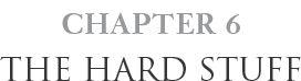
I'll start with a different example expanded from chapter 3. A Bayesian analysis of a drug's efficacy will ignore such contingencies as the name of the scientist who will observe and report the results. But technically we might object to that, since “result x will be reported by Dr. Smith” and “result x will be reported by Dr. Jones” are two different outcomes, and thus in each case we have a different e, one in which we have data from Dr. Smith, and another in which we have data from Dr. Jones. We therefore cannot say e is, for example, 100 percent likely if h is true (i.e., that hstrongly predicts e) when we could have had a different e, i.e., we could have data from Smith instead of Jones. If the hypothesis is that the drug will always show outcome x, we obviously want to say P(e|h.b) = 1 when e = x, but that's impossible when ‘x from Smith’ and ‘x from Jones’ are mutually exclusive, yet both outcomes are equally possible on h (just as countless different configurations of the stars are possible on the Big Bang Theory). Since e is always one or the other (i.e., either from Smith or from Jones), and nothing in h entails one over the other (i.e., neither scientist's being the observer is more likely), at the very least P(e|h.b) should be 0.5 for each possible outcome (either an observation of x by Smith or an observation of x by Jones). But the number of possible scientists is factually in the thousands, and in hypothetical extension approaches infinity (i.e., there are infinitely many “Dr. Z saw x” outcomes that are logically possible yet would still fulfill the prediction of h, and as shown in chapter 2, page 23, nearly everything that is logically possible has a nonzero probability).11 So, too, the configuration of the stars.
It seems intuitively obvious that this is ridiculous and that we're right to ignore these contingencies, but on close reflection it's not immediately clear why that intuition is correct (which I suppose explains those mathematicians who scoff when I suggest it). The justification is fairly simple, however. Since h actually makes no predictions regarding who will make the observations and who won't, the coefficient of contingency will be the same for both consequent probabilities. For example, assume the probability is n that x will be observed by Smith rather than any other of the thousands of scientists who realistically could have been in her position, and that the probability that x will be observed if h is true is otherwise 1 and the probability that x will be observed if h is false is otherwise (let's say) 0.2, and that the priors are equal. Then on some scientist observing xthe completed formula would be:
The coefficient n thus cancels out. It vanishes from the final equation. It therefore never needed to be introduced in the first place. This is because any probability that, say, Smith is more likely to have observed e is the same whether h or ~h and therefore “the probability that e would be observed if ~h” is multiplied by exactly the same probability (that it would be Smith instead of Jones who saw e) as “the probability that e would be observed if h.” Since it's just as likely that Smith would be the one to observe e whether h or ~h, it doesn't matter what the likelihood is that Smith is the one to have observed e (and, as here shown, Bayes's Theorem proves this). Just as this is true for the exact name of the scientist who makes the observations that become e, it's true of every other contingency of whatever kind (such as exactly which configuration the stars are in), so long as h makes no specific predictions regarding it.
This is related to the converse tactic of adding ad hoc elements to a theory (discussed in chapter 3, page 80), for example, the probability that e (‘Jones was shot five times in the head’) given h (“Jones was murdered”) remains virtually 100 percent regardless of who committed the murder. Any more specific theory such as “Smith murdered Jones” would not reduce that probability. It would remain virtually 100 percent (assuming there is no other pertinent evidence). But specifying such a theory will reduce the prior probability, because that must be divided among all possible suspects (see my example of assassination theories on page 227). But this is only because specifying the murderer is now a component of h. In the case of contingencies like whether Smith or Jones observed the e that was predicted by h, the specification of who would make the observation is not a component of h, and therefore no reduction of the prior probability ensues (for exactly the reasons already explained in chapter 3: the prior probability that it was “Smith or Jones” equals the sum of the prior probabilities of every relevant possibility, e.g., “only Smith,” “only Jones,” and “Smith and Jones”; yet h predicts only “Smith or Jones,” which includes all of the above). Yet the consequent probability also remains the same. So this contingency has no effect at all.
Thus, per the example I used in chapter 3 (page 77), if h is a theory of the origins of Christianity that makes no predictions regarding which exact name the Gospel of Mark would be assigned, but only predicts that it would be assigned some name (or indeed, doesn't even entail anything about whether it would or wouldn't be named at all, only that it would be written), then we don't have to concern ourselves with the probability that the name would be Mark. And this follows all the way down the line, for example, h doesn't even have to predict specifically that that Gospel would be written, but only that some sacred story about Jesus would have come to exist conveying at least the information h entails was paramount to early Christians, which prediction could be satisfied by a largely different text than was actually produced. Also, sometimes even when h does make one name more likely than another (or one text more likely than another, or anything more likely than another), it may do so to such a slight degree (warranting only a small difference in probability either way) that the difference is washed out by a fortiori estimates and thus can be ignored anyway (this phenomenon of a fortiori estimates “washing out” small probabilities was explained in chapter 3, page 85).
This has broad epistemological importance. Just as ‘exactly by whom and exactly when’ is not normally a predictive component of h in any scientific experiment, so ‘exactly what’ is not normally a predictive component of h in any historical theory. This goes beyond irrelevancies entailed by our background knowledge. For example, we can formulate an h about Jesus that only entails three specific things would be said about him, regardless of how, in what medium, or in conjunction with what else. Such an h renders the appearance of those three things highly probable in any surviving text about Jesus from that period, of whatever sort, without entailing anything else about what those texts would be or say. Thus, we needn't calculate the odds that the Gospel of Mark would be produced, word for word, exactly as we have it (which odds would be astronomically small, given all the possible configurations of words that could convey the same things). No hypothesis usually makes any predictions regarding such specifics, and thus any coefficient of contingency accounting for them would identically affect both consequents, and thus would mathematically cancel out. Only, of course, if a hypothesis did make a differential prediction regarding such details would the coefficient of contingency entailed have to be accounted for, and even then only if the difference was large enough to matter. The method of emulation criteria (analyzed at the end of chapter 5, page 192) is in effect a miniature example of that, where one hypothesis proposes certain components of a text are there by chance (either the chance decisions of the author or the chance coincidences of history), but another proposes those components are there by design (comparable to the stars being in that eerie cross pattern suggested earlier). But even then (as I discussed before) a hypothesis of design rarely makes exact predictions, but rather generic predictions that are merely more exact than a hypothesis of chance would entail. In other words, like the Big Bang Theory and the arrangement of the stars, you can formulate a hypothesis that only makes predictions regarding general characteristics. This is just as true in science. For example, a scientific hypothesis can predict the general pattern of events to expect from a volcanic eruption, without predicting exactly what will happen (such as which direction ash will drift, because that will be contingent on factors unrelated to volcanoes, such as the prevailing wind at the time).
But sometimes the solution pertains to the role of b, rather than the structure of h. In chapter 3 I began by comparing two examples—a hypothetical darkness in 1983 and a purported darkness in the 30s CE—and one factor that came up was the fact that so much evidence survives from 1983, whereas evidence that survives from antiquity has passed through a highly destructive and largely random filter. The hypothesis h “Jesus was executed by Pontius Pilate” (in conjunction with our background knowledge b) entails that an official record of the trial and verdict was created and filed in the Roman archives of Caesarea. If Jesus had been tried and executed in New York in 1983, the same would have occurred. Yet if we pored through court archives from 1983 and found no trace of that trial, this would substantially lower P(e|h.b), because h predicts evidence that didn't turn up. Yet surely not having the same court record from the time of Pilate shouldn't lower P(e|h.b) at all, because (given our background knowledge) we have no reason to expect that record to survive. And yet h does not entail the prediction “an official Roman record of the trial would not survive,” that is, h does not predict the absence of that court record. Indeed, if next year we found a stash of official first-century documents buried under modern Caesarea that included exactly that trial record (and the find was fully authenticated), we would count this as greatly increasing the probability that h is true (so enormously, I suspect, that h would become an unassailable certainty). And yet h cannot be stated as predicting we would find that record, because then our not having found that record would have to reduce P(e|h.b), indeed quite substantially (in fact, by exactly as much as having that record would increase it).
This problem ranges far beyond this one example. Nearly every hypothesis about antiquity entails the existence of vast quantities of evidence next to none of which survives or was even expected to have survived—or in fact none survives at all, and wasn't expected to. But this already follows from the fact that consequent probabilities are conditional on both h and b, and b entails our knowledge of the scarce and random survival of ancient evidence like this. So the difficulty is easily resolved in the logic of BT. The probability that Pilate's “record of the trial” would survive is small, due to the contents of b, but that does not mean P(RECORD IS FOUND|h) is small (and therefore finding it would reduce (!) the epistemic probability of h). That's because h entails P(RECORD IS FOUND|h) is very high only given the record's survival (through the usual destructive filter all ancient evidence has passed through), and the outcome of that contingency is not entailed by h (as long as h makes no prediction whether that record will have survived that filter), so if the record turns up (and thus survived the filter after all), its discovery should still increase the epistemic probability of h as expected.
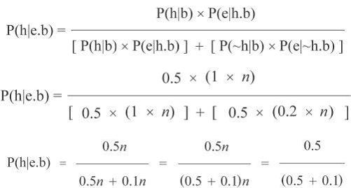
Thus, making the consequent probability also conditional on b is what makes the difference here (hence in BT this probability is in fact P(RECORD IS FOUND|h.b) and not just P(RECORD IS FOUND|h)). So, either the record existed or it didn't; h predicts that it did; but b entails that even if it did, it probably didn't survive (note that h does not entail this, only b does—at least in this example). This circumstance is analogous to the ‘trustworthy neighbor’ example in chapter 3 (page 74). If R = ‘the record existed’ and F = ‘such a record would have been found by now,’ then I'll assign these arbitrary numbers just for the sake of argument:
P(F|R.b) = 0.01 […which entails…] P(~F|R.b) = 0.99
P(F|~R.b) = 0.001 […which entails…] P(~F|~R.b) = 0.999
You might think P(F|~R.b) = 0, since if it didn't exist, obviously it won't have been found, but there is a nonzero probability of forgeries and erroneously filed records. In other words, just because we find such a record does not automatically entail h is true, because the record we find may be a forgery or may have been filed erroneously in the first place (and of course there are all the more extreme possibilities, such as that we're hallucinating our finding the record—but those usually have vanishingly small probabilities). Thus I assign P(F|~R.b) = 0.001 to reflect these possibilities (though to have such a low probability requires the record to survive a reliable process of authentication, since forgery is so common, particularly in the field of biblical antiquities).
It's also true that apart from the filter, I'm assuming P(R|h.b) equals one, even though usually it will be something less than one, for example, there is always some small probability that an official record that would usually be made and filed didn't get made or filed, but that probability is often small enough to ignore. Likewise, if there is any chance we would know, if the record didn't exist, that it didn't exist (as sometimes is the case, e.g., there is always some small probability that someone in antiquity would have checked and reported it didn't exist, and that report could have survived), that would also have to be factored in, but again this probability may be so small that it can be ignored (see my analysis of the Argument from Silence in chapter 4, page 117). Conversely, it's also possible to have such a report about the record that is itself a lie or in error, thus even having a report of the record's nonexistence would still not strictly entail the record didn't exist, requiring an estimate of probabilities again (likewise for a report that claimed it did exist). I will ignore all these possibilities here (and assume instead that h strictly entails R and that ~hmakes no predictions other than ~R). But I make a point of noting all this here because sometimes such factors will have a large enough effect that they cannot be ignored.
You might then object to my assignment of P(~F|~R.b) = 0.999 since if the record didn't exist, our not having it is still not so certain—for we could have turned up a forgery or an administrative error by now. But P(~F|~R.b) must reflect the actual probability of a forgery or administrative error—which is not their probability given that the document is found, since given that the document isn't found the probability that we should still expect such a document to have been erroneously or deceitfully produced by now is not the same. In fact, the latter is usually vanishingly small. Hence I could even assign P(~F|~R.b) = 1 as a practical stand-in for P(~F|~R.b) → 1, which reflects the assumption that such forgeries and errors are rare enough that we shouldn't ever expect them to exist (as if every bogus item of evidence conceivable had been forged by now)—whereas we do have grounds to suspect forgery when a suspiciously convenient document actually turns up, and for that reason I did not allow P(F|~R.b) = 0. Technically this forbids P(~F|~R.b) = 1, since it is necessarily the case that P(~F|~R.b) = [1 – P(F|~R.b)], and therefore must be 0.999 if P(F|~R.b) = 0.001 (since given ~R the alternatives F and ~F exhaust all possibilities, and therefore their respective probabilities must sum to 1). But the difference between 1 and 0.999 is too small to matter in the present case (whereas the difference between 0 and 0.001, in fact any nonzero number, is effectively infinite). So I will use 1 only to simplify the math, because that won't change the outcome in any visible way.
Given these numbers, then a Bayesian analysis that hinged solely on this piece of evidence would go as follows. If the record is not found (the state of evidence we are actually in) and if h entails R and (let's say) P(h|b) = 0.9 (i.e., we are otherwise convinced h is probably true) then:
So the absence of the record does reduce P(h|e.b), from an initial belief of 0.900 to a revised belief of 0.899, but this change is so little as to make no practical difference. In fact, since P(F|R.b) should really in this case be far lower than 0.01 (i.e., the probability we'd have Pilate's court records is surely far less than one in a hundred, indeed probably less than one in a million), the effect of the missing evidence is really even smaller, in fact so small as to be effectively invisible. Hence we can ignore it. So our intuition that the absence of this evidence should not lower P(e|h.b) “at all” was technically wrong but in practice correct; we just don't have any convenient vocabulary to express “as near to not lowering it at all as is practically the same as not lowering it at all” so we revert to “not at all” because our intuitions tell us that's close enough. Only when we don't have an extremely high expectation the evidence would be lost would that not follow (hence my analysis of the Argument from Silence in chapter 4, page 117).
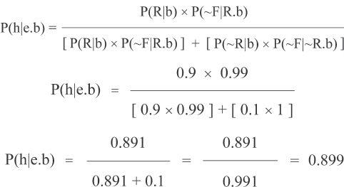
Meanwhile, if the record is found:
Thus finding the record does increase P(h|e.b), exactly as expected, from an initial belief of 0.9 to a revised belief of 0.989, representing a rather large increase in our confidence that h is true. Which is all as we intuited should be the case.
These analyses can be repeated for any other comparable case, where we can't predict from h exactly what evidence we would now have, either due to h itself entailing nothing either way (except at most in some general respects) or due to b entailing a change of expectations from what they'd be given h alone. Thus, that being a fact does not impair historical reasoning at all, and any philosophers or mathematicians who've ever worried about this can rest easy. For example, McCullagh discusses an example in which a very different type of contingency played a role: an event occurred in a private household, which just happened to be witnessed and recorded in a diary by a traveling Frenchman, allowing us now to argue that the event occurred by appealing to the evidence of his diary.12 And yet our h (“the event occurred”) in no way predicts that there would have been a traveling Frenchman just happening by. That is actually very improbable, hence our evidence is very improbable. Yet surely its being improbable should not lower the probability of h. To the contrary, such evidence should increase that probability, quite substantially in fact. In other words, if M = ‘that Frenchman happened by and wrote in his diary what he saw’ and V = ‘that event happened,’ then (all else being equal) P(V|M) should be high. But h only predicts V, not M, while b entails M is very improbable. Here we'll assume h entails V, so in BT we are only concerned with determining P(V|e.b), and if we assume M constitutes e (we actually have the Frenchman's diary, and that's all we have), then P(V|e.b) = P(V|M.b), which produces:
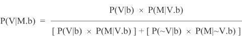
If we split M into D and F, D = ‘diary entry attesting V’ and F = ‘Frenchman happened by,’ and assume P(V|b) = 0.5 (i.e., we have no prior reason to suspect V either did or didn't happen), and that the Frenchman happening by has a contingency coefficient of n (representing the improbability of that coincidence, i.e., P(F|b) = n), and if we assume that P(D|V.F.b) = 0.99 (i.e., if when we assume F and V, then the odds we'd have the diary entry are nearly 1; yes, the further contingency of the Frenchman, given his being there, recording the event, could similarly be analyzed, but that would take the same form as the contingency of the Frenchman being there, and thus that analysis would look essentially the same as the following) and if we assume that P(D|~V.F) = 0.01 (i.e., if when we assume F and ~V, then the odds we'd have the diary entry are 0.01, i.e., the small probability the Frenchman would make the story up), and if we assume, of course, that if ~F, then ~D (so both P(D|~V.~F.b) and P(D|V.~F.b) = 0, i.e., if the Frenchman didn't happen by, the diary entry wouldn't exist, and therefore ~M), then:
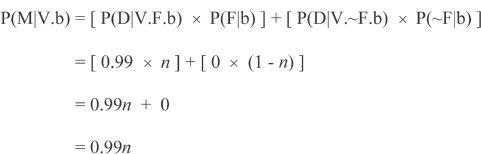
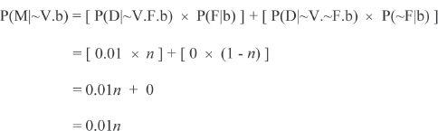
So:
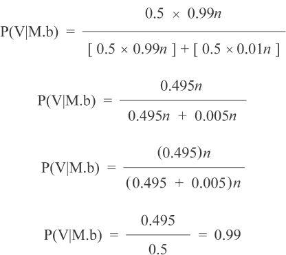
As before, the coefficient of contingency cancels out and thus disappears, making no difference to the outcome. As expected, given the assigned probabilities, the existence of the diary entry greatly increases the probability that the event happened. The extreme improbability of a Frenchman just happening by is completely moot.
Other concerns about contingency are already resolved by probability theory. For example, sometimes it's claimed that the probability of life arising on earth is very small, whereas if it was by design, the odds would be very high, creating such an enormous disparity in consequent probabilities that unless you have a wildly outrageous bias against the existence of a Creator (resulting in an extraordinarily large disparity in the priors against it), BT entails life was created by intelligent design. But there are two fallacies in this argument. The first is of invalidly predicting efrom h, when in fact from the hypothesis “God exists” it isn't possible to deduce the prediction ‘simple, single-celled carbon-coded life forms would arise on just this one planet out of trillions, and only billions of years after the universe formed, which would only slowly evolve into humans after billions of years more’ etc. Thus P(e|GOD.b) in this instance is not ‘very high.’ In fact, arguably it's extraordinarily low, even before adding any background knowledge that renders such divine beings improbable in and of themselves.13 The second fallacy, however, is a common mistake in reasoning about probability: the odds of life forming by chance are not the odds of life forming by chance specifically here on earth, but the odds of life forming by chance on some planet somewhere in the whole of the known universe.14 Because, obviously, wherever that happens to be will become “specifically here” for whoever ends up evolving on that planet to think about it. It's the difference between you winning the lottery (which is very improbable) and someone winning the lottery (which is very probable). You are reasoning fallaciously if, after winning, you conclude the lottery must be rigged simply because your winning was so very improbable. Because someone was likely to win, and that someone was as likely to be you as anyone else playing. Hence, in fact, the number of planets and years available are such that, where L = ‘life as we observe it to be’ and U = ‘the universe as we observe it to be,’ P(L|U)→1. And since (as suggested earlier), P(L|GOD)→0, the consequent probabilities are in fact exactly the reverse of what was thought, such that even if P(GOD|b) were high (and it's not), life still probably wasn't created by intelligent design.15
The relevance of this to history is that the same kind of fallacious arguments can arise if you do not attend to the correct probabilities. For example, you cannot argue that Alexander the Great assassinated his father Phillip because the odds of that assassination happening by chance are small, but the odds of that happening “if Alexander did it” approach certainty. To begin with, such coincidences happen all the time (often kings are assassinated who just by chance have sons or successors who will benefit; indeed, this is probably true in most cases)—so the probability that this is one of those coincidences is actually high, not low (I'll discuss this phenomenon using a poker analogy on page 254). But more importantly, in Bayesian analysis this doesn't even become an issue because ~h would have to be accounted for, in which we would list a number of known persons who had the same motive (and that's assuming we can leave out of account the many unknown persons who would also have motive), and the prior probability for each being the culprit would have to be the same (assuming we have no other evidence implicating Alexander, or any one else), and, more importantly, the consequent probability would be the same for all of them. That is, “Phillip gets assassinated” is 100 percent certain on any “x did it” hypothesis. So Alexander is no more likely to be the culprit than anyone else. In other words, it's fallacious from the start to assume the hypothesis “Alexander did it” is competing against “chance” (as if random quantum events caused kings to be assassinated). Rather, it's competing against other assassins, for every one of whom “the odds of Phillip getting assassinated” are 100 percent. Of course, if we have other evidence, then e is not just “Phillip got assassinated” but the conjunction of all that evidence, which could implicate someone specific. Or if there were no other known suspects (or the only known suspects are actually only known from Alexander claiming they are suspects), the prior probability could favor Alexander. If a study of royal assassinations found that, statistically, sons more likely turned out to be the culprit, or that, when there was only one known suspect, more often than not they turned out to be the culprit, such data could be used to alter the priors (if all the contexts are sufficiently similar—see my following discussion of using reference classes to assign priors).
That's just one example. Many more can be imagined. All the scenarios above support the same conclusion: most contingencies can be ignored, and hypotheses can validly make generic predictions exactly as argued in chapter 3. And contingencies that can't be ignored can be fully accounted for in BT.
DETERMINING A REFERENCE CLASS
Strictly speaking, prior probability is the probability of getting a specific kind of h when you draw at random from a reference class of all possible h → e correlations. Those correlations don't have to be causal, although in history they usually are. Because, in history, we are almost always asking what caused e and proposing h as the answer (see chapters 2 and 3). I'll thus focus mainly on causal hypotheses and explain how to ascertain prior probabilities in a way that can produce intersubjective agreement among expert historians, and when and why such a process is logically valid.
Some critics of BT are skeptical of causal language in applying the theorem, but that's fundamental to many theories, especially historical ones, since any statement about what happened in history reduces to a statement about what caused the evidence we have. And you can't propose historical explanations without proposing causes. Historians do distinguish claims about what happened (or once existed) from claims about why it happened (or why it existed). But ultimately all claims about ‘what’ entail claims about ‘why.’ For example, we can talk about what the frequency of a particular name actually was in Roman times by talking about the frequency of that name in inscriptions, but that entails assuming a causal relation between actual name frequencies and the appearance of names on inscriptions, whereas merely talking about the frequency of names on extant inscriptions, without any interest in what caused this frequency, is all but useless to a historian, not only because you must assume actual name frequencies is what caused the inscribed name frequencies, but especially because even the claim that these inscriptions are ancient entails an unavoidably causal theory about how they came to exist, and for a historian to disregard even the question of whether Roman inscriptions are ancient (or even Roman) is simply an abandonment of history as a field of inquiry.
This remains the case even when the causal relationship appears the other way around. For example, a hypothesis of murder will explain evidence of preparations for that murder, even though the murder didn't “cause” that evidence (since the preparations preceded the murder). Yet the hypothesis still entails there is a causal relationship between the murder and the preparations: in this case, the intent to murder, which is inherent in that hypothesis, will have caused both. Similarly, a hypothesis that a religious riot was caused by prior beliefs of that community (such as an ancient prophecy) in conjunction with new events (such as the appearance of a comet) obviously proposes a causal relationship between those prior beliefs and the riot, but not that the riot caused those beliefs. That the prior beliefs existed is evidence supporting the hypothesis (which is that “they rioted because of that ancient prophecy”) and therefore this hypothesis makes that evidence more probable, even though the riot did not cause that evidence, but the other way around (the prophecy, in part, caused the riot—the very causal relationship being hypothesized).
Formally speaking, if the riot occurred because of that prophecy, then the probability that there would be no such prophecy (or P(~e|h.b)) is zero, so the consequent probability (or P(e|h.b)) of that item of evidence is 1 (because P(e|h.b) always equals 1 – P(~e|h.b), a useful observation I'll discuss on page 255). In other words, on that hypothesis, the existence of the prophecy is exactly what we should expect (in fact, if the hypothesis were true, the absence of that evidence would be impossible—apart, of course, from the contingency of that evidence being lost, as we discussed earlier in this chapter). On the other hand, if the riot did not occur because of that prophecy (in other words, if ~h), then the probability that there would be no such prophecy (or P(~e|~h.b)) is not zero, and therefore the consequent probability (or P(e|~h.b)) of that item of evidence is less than 1. Because then, it is not exactly what we would expect to be in evidence (even if it's not wholly unexpected). Of course, if ~h is the hypothesis that the absence of the prophecy caused the riot, then P(e|~h.b) is not only less than 1 but in fact nearly zero, since the prophecy is in evidence, and that is exactly the opposite of what that hypothesis predicts (the consequent only escapes not being zero because of such possibilities as that the prophecy existed but no one knew about it or that the prophecy was fabricated after the riot). But still we are talking about a causal hypothesis, whether it's a hypothesized event causing the evidence, or the evidence causing the hypothesized event. Or, as in the case of name frequencies on inscriptions, we are talking about a fact assumed by a hypothesis causing the evidence: that a particular frequency of names in ancient Rome caused the frequency of names on surviving inscriptions.
Thus all historical claims that Bayes's Theorem can ever test must involve causal hypotheses, which link the claim to the evidence. But those causal hypotheses need not always be fully specified. For example, if (let's say, with a sample size in the hundreds) archaeology confirmed 8 out of 10 Roman colonies (cities established by the Roman government for settling war veterans) had public libraries, we could use that as a prior probability that a newly excavated Roman colony had a public library, without specifying the exact causal relation that produced this probability. We are still implicitly assuming there is one, that is, something caused Romans to regularly fund public libraries in their colonies and something caused them not to from time to time, but we don't need to know what either “something” was, since whatever those “somethings” were, we already know what frequencies of outcome they generated, and that's all we need in this case. Certainly, if we acquire information regarding those causes, then that information becomes relevant again (hence it's worth repeating here that the results of BT are always conditional on current knowledge—when we get new information, those results may change, the epistemological significance of which I'll discuss later on page 276). For example, if we discovered that certain specific families were responsible for funding most of those libraries, we might be able to revise our probabilities accordingly. If what caused most of those libraries was the patronage of those wealthy families, such that all the identified colonies that received their patronage had libraries, and only 2 out of 10 other colonies had libraries (let's say, because the veterans settled in those 2 in 10 cases had the means and interest to combine their own resources to establish a library to bring more prestige to their colony), then if the colony we are newly excavating can be independently determined to have received patronage from those identified families or not, our priors can be revised. If our city is determined to have had that special patronage, and our data shows 67 out of 67 cities with their patronage have public libraries, then the prior probability our new city did as well will now be over 98%.16 Of course that assumes the evidence establishing this city had their patronage is so strong that the probability of that connection is extremely high, high enough that the odds of our being wrong about it make no discernible difference to the result. But that aside, what we get is 98%, which is a lot higher than the 80% we were working with before. Hence with better information we get better estimates. Likewise, if our city is determined not to have had that special patronage, and assuming all else is the same, then the prior probability our new city had a public library will only be about 20% (2 in 10), or perhaps closer to 21% (see note 16, page 326). Again, better information, better estimate.
This is what is called a reference class. In that last case, the reference class is ‘Roman colonies lacking special patronage,’ whereas in the preceding case the reference class is ‘Roman colonies receiving special patronage,’ which two classes are mutually exclusive, but both comprise a larger reference class of just ‘Roman colonies.’ If all we know is that a city we are excavating falls in that last (combined) reference class, then we must use the prior probability that that class entails. Only if we know it falls into one of those more specific sub-classes can we use the prior probabilities that those classes entail. The challenge of ascertaining prior probability always reduces to this same exercise of determining the most relevant reference class (for which we have, or can hypothetically construct, credible frequency data). Imagine you can put all cases into a hat (even the ones we don't know about yet) and scramble them up and then draw one of them from that hat at random. The prior probability that a new case will exhibit the relevant feature corresponding to h equals the chance of drawing it out of that hat. For example, following the previous example, if we put all Roman colonies into a hat and drew one at random, we'll draw a city with a public library out of that hat an average of 8 out of every 10 pulls, making the chance of such a draw 80%. Hence the prior probability is 80%.
Many object that there is rarely any objective way to settle on how to determine the prior probability, because any given hypothesis will simultaneously belong to countless reference classes, and which reference class you use to develop the prior can seem rather arbitrary.17 But when two parties come up with different ways to determine the prior probability (because, as John Earman says, “there are different ways of conceptualizing an inference problem” in Bayes's Theorem, just as in any other method), we must ask whether party A's prior is based on more or less information than party B's. Is A's reference class narrower or better understood than B's? If the answer is yes, then party A's prior is to be preferred, and vice versa. To do otherwise would be to willfully ignore information, as if we know a Roman colony had special patronage, yet used the broader reference class of ‘all Roman colonies’ anyway. That's a violation of the logic of BT, which requires the prior probability to be conditional on b, and the fact that our case falls into a narrower reference class is information in b. In effect, we know the prior probability in this case is 20% and not 80%, and BT entails we must use what we know. I call this the rule of greater knowledge. When we know more, our estimates must reflect that greater knowledge. We can't pretend we don't have it.
If, on the other hand, the two competing reference classes are epistemically equal, and we don't know what's in the sub-class that is a conjunction of those two competing classes, then the problem of selecting the reference class gets more complex. For example, suppose we are excavating a newly discovered Roman colony in Italy named Seguntium, and we want to argue that a building we've uncovered is a public library, and we have our consequent probabilities worked out, but we need to determine our priors. Suppose, also, that we already know to a very high probability that it is such a colony and it did not have special patronage, and that we also know colonies in Italy had public libraries at a rate of 90% instead of the 80% rate more generally. We now have two different reference classes, each giving wildly different estimates of prior probability: the ‘no patronage’ class at 20% and the ‘in Italy’ class of 90%. Ordinarily, of course, with the kind of data imagined for this scenario, the frequency of public libraries in the reference class ‘Roman colonies in Italy without special patronage’ would also be known, and would necessarily supersede all others (per the rule of greater knowledge, establishing the logical requirement of preferring the narrowest available sub-class, and here we would have a proper sub-class produced by the conjunction of the competing classes ‘without patronage’ and ‘in Italy’). But it's possible we never found adequate information to establish or rule out the ‘special patronage’ in any of the other Italian colonies, and thus we can't determine the statistical content of the reference class ‘Roman colonies in Italy without special patronage.’ We're then stuck with two equally applicable reference classes that give entirely contradictory indications of the prior probability.
In such a circumstance, the simplest solution might be to generate a conclusion with an upper and lower bound, thereby using both reference classes (the ‘no patronage’ class giving us the lower bound and the ‘in Italy’ class giving us the upper bound). If there were many more simultaneously competing classes, one would use the two that entail the highest and lowest priors since the resulting span will thus encompass all the others anyway. But that solution is often incorrect (as the true prior could well be outside the resulting range) or renders results too ambiguous to be of any use. Usually we should prefer one class over the other (and in this example we should, as I'll explain on page 238).
In reality, of course, there still is a sub-class ‘Roman colonies in Italy without special patronage’; it's just that in this example we don't know what's in that class, forcing us to guess, thus introducing a wider margin of error. For example, the difference between the Italy class and the more general class (‘all Roman colonies’) of 90% rather than 80% having libraries, may be entirely the result of more colonies in Italy receiving that special patronage than elsewhere (in which case the reference class ‘colonies without patronage’ would be the more accurate class and our prior should be 20% and not 90%). But it might also be the result of veteran settlers in Italy being wealthier than elsewhere and thus funding more libraries on their own, in which case the reference class ‘all colonies without patronage’ would be the wrong class, because the narrower ‘colonies without patronage in Italy’ entails a different prior probability, perhaps 30% instead of 20%, in any case some higher frequency presently unknown to us due to our lack of information. Or there could be any of countless other possibilities. Of course, just as in the case of ‘all colonies’ vs. ‘colonies without patronage,’ we should prefer the more general class when we don't know the frequency in the sub-class, so we should here, too, and thus prefer the more general class ‘colonies without patronage’ until we know more about the sub-class ‘colonies without patronage in Italy.’ I'll say more about why later (page 238). But until we have actual information regarding such possibilities, we may have to accept the huge range of uncertainty entailed by the two reference classes we can identify but can't pare down.
And for all that, it's still possible the conjoined class entails a lower or higher prior probability; for example, if for some reason all ‘colonies without patronage in Italy’ have no libraries, or if for some reason all of them do (or any other frequency). It's just that we have no information that makes either likely. That is, given the information we have, we should expect 2 in 10 ‘colonies without patronage’ to have libraries, not (for instance) 10 in 10, or 0 in 10, even in Italy. In other words, until we know otherwise we have to assume the frequency for the whole region applies to each sub-region. The mere possibility that things could be different in Italy does not warrant assuming they are (hence my fifth axiom in chapter 2, page 26). We might later be able to prove otherwise, but until then we must base our assumptions on what we now know. This is logically required by BT. And when our knowledge indicates two different possibilities, we have to allow either to be the case until we can narrow it down (and as it happens, in this case we can, as I'll show on page 238). And, of course, if we also rely on a fortiori estimates we'll be on even safer ground (see chapter 3, page 85).
The following Venn diagrams illustrate the four most common conditions of competing reference classes:
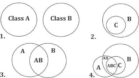
Condition 1 can never produce a valid conflict. If two reference classes actually apply to the same hypothesis, that fact logically entails their conjunction (since at the very least, their conjunction will contain our hypothesis—provided our hypothesis is logically possible). Thus, when faced with Condition 1, we need only ascertain which reference class applies to our h, A or B. Condition 2 is more typical, a case of narrowing the reference class. If our hypothesis resides in Class C and we can derive a prior probability from that class, we must do so. Because knowing h resides in C constitutes more information about h than is entailed by B alone. Condition 3 is also common, and similar to Condition 2. If our hypothesis resides in Class AB and we can derive a prior probability from that class, we must do so. Because knowing h resides in AB constitutes more information about h than is entailed by either A or B alone. If, however, we cannot derive a prior from that sub-class (because we lack the requisite data for it), and the priors entailed by A and B differ, we can conclude the prior probably falls somewhere in between (unless we have definite knowledge already that their conjunction would change that expectation, e.g., carbon, sulphur, and potassium nitrate each have low probabilities of catching fire, but their conjunction has an extremely high probability of that, thus the combined class takes on properties well outside the average of the individual classes due to the causal interaction of the parts—and as in chemistry, sometimes also in history and social systems). But we can often get more specific than that. As I'll explain in a moment, there are some logical shortcuts we can take to show that the prior more probably falls nearer one side than the other (we can even apply sophisticated techniques in probability calculus on the complete set of data to get essentially the same results, but that's beyond the scope of the present book). Finally, Condition 4, exemplifying a more complicated case, simply combines the circumstances of Conditions 2 and 3.
The actual statistical problem created by the Seguntium example could become very complex and might have to take into account many other variables. Historians rarely face such problems, and even more rarely have the skill set to solve them (although they can always collaborate with mathematicians, and arguably sometimes should). But historians do need some simple rules of their own for rationally negotiating complex cases that have little or no exact data. To illustrate this, the libraries scenario can be represented with this Venn diagram:
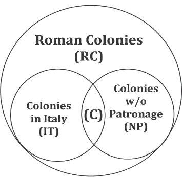
In this example, P(LIBRARY|RC) = 0.80, P(LIBRARY|IT) = 0.90, and P(LIBRARY|NP) = 0.20. What's unknown is P(LIBRARY|C), the frequency of libraries at the conjunction of all three sets. If we use the shortcut of assigning P(LIBRARY|C) the value of P(LIBRARY|NP) < P(LIBRARY|C) < P(LIBRARY|IT), that is, P(LIBRARY|C) can be any value from P(LIBRARY|NP) to P(LIBRARY|IT), then the first concern is how likely it is that P(LIBRARY|C) might actually be less than P(LIBRARY|NP), or more than P(LIBRARY|IT), and the second concern is whether we can instead narrow the range. Given that we know Seguntium lacked special patronage, in order for P(LIBRARY|C) < P(LIBRARY|NP), there have to be regionally pervasive differences in the means and motives of veteran settlers in Italy—enough to make a significant difference from veteran settlers in the rest of the Roman empire. And indeed, on the other side of the equation, for P(LIBRARY|C) > P(LIBRARY|IT) these deviations would have to be remarkably extreme, not only because P(LIBRARY|IT) > P(LIBRARY|RC), but also because P(LIBRARY|RC) is already >> P(LIBRARY|NP), which to overcome requires something extremely unusual. Lacking evidence of such differences, we must assume there are none until we know otherwise, and even becoming aware of such differences, we must only allow those differences to have realistic effects (e.g., evidence of a small difference in conditions cannot normally warrant a huge difference in outcome; and if you propose something abnormal, you have to argue for it from pertinent evidence—which all constitutes attending to the contents of b and its conditional effect on probabilities in BT).
However, we would have to say all the same for P(LIBRARY|C) > P(LIBRARY|NP), since we have no more evidence that P(LIBRARY|C) is anything other than exactly P(LIBRARY|NP). All we have is the fact that P(LIBRARY|IT) is higher than P(LIBRARY|RC), but that in itself does not even suggest an increase in P(LIBRARY|NP), and certainly not much of an increase. Thus P(LIBRARY|NP) < P(LIBRARY|C) < P(LIBRARY|IT) introduces far more ambiguity than the facts warrant. There is every reason to believe P(LIBRARY|C) ≈ P(LIBRARY|NP) and no reason to believe being in Italy makes that much of a difference, especially as P(LIBRARY|IT) is only slightly greater than P(LIBRARY|RC), which does suggest only a small rather than a large difference between Italy and the rest of the empire, and likewise we should expect the large disparity between P(LIBRARY|NP) and P(LIBRARY|RC) to be preserved between P(LIBRARY|C) and P(LIBRARY|IT), as the causes producing the first disparity should be similarly operating to produce the second—unless, again, we have evidence otherwise. In short, NP appears to be far more relevant a reference class than IT in this case and should be preferred until we know otherwise. And if we also use a fortiori values (setting the probability at, say, 10–30%), we will almost certainly be right to a high degree of probability. All this constitutes a more complex application of the rule of greater knowledge. When you have competing reference classes entailing a higher and a lower prior, if you have no information indicating one prior is closer to the actual (but unknown) prior, then you must accept a margin of error encompassing both, but when you have information indicating the actual prior is most probably nearer to one than the other, you must conclude that it is (because, so far as you know, it is). In short, we can already conclude that it's so unlikely that P(LIBRARY|C) deviates by any significant amount from P(LIBRARY|NP) that we must conclude, more probably than not, P(LIBRARY|C) ≈ P(LIBRARY|NP), regardless of the difference between P(LIBRARY|IT) and P(LIBRARY|RC). And as in this case, so in many others you'll encounter.18
All the same follows even when such precise and abundant data is not available to determine priors. We often have to assess a theory's relative plausibility subjectively in light of a kind of holistic polling of our background knowledge (the logic of which I'll discuss in the next section, starting on page 257). If we stick to a fortiori reasoning, and do our best to ensure we are honest and discerning when polling our background knowledge, and as long as we are as well informed as we reasonably can be in the circumstances, then this will still produce better-than-arbitrary results, in fact often entirely reasonable and defensible results. After all, that's why any knowledge of the past is possible. It's also why expert opinion carries greater weight (as argued in chapter 2): as far as analyzing claims in their own field, experts have seen more relevant data and thus can get more informed results when holistically polling their past experience. But this still requires actual confirmed experience, not past hunches. In other words, it requires data that can be communicated, shared, or repeated by others, which means ultimately an expert must be able to adduce many actual examples confirming his statistical opinions in general when called upon to justify his estimates, and if he cannot, then his estimates are not justified or are too weakly justified to carry any special weight.
Sometimes a competing reference class becomes moot. As noted in chapter 5 (page 168), we can run a series of BT arguments by starting with a neutral prior (0.5) and then run a single case, then run another case using the outcome of the first case (i.e., its posterior probability) as the prior in the second case, and so on down the line until we've exhausted all known cases capable of analysis. The end result will be the correct Bayesian conclusion (the correct epistemic probability of h in light of all evidence e and all background knowledge b).19 And sometimes when there are two competing reference classes, both of them will get picked up eventually in this series, and thus it won't matter which one we start with (since mathematically the outcome will be the same, just as it doesn't matter whether we multiply 6 × 5 or 5 × 6, you still always get 30). This is not the case for the Seguntium example (because the competing classes in that case are not equal, i.e., upon analysis only one of them was found likely to be close to the actual reference class). But it can happen. We could divide any body of evidence into two and derive a prior probability from one of them and use the other to develop the consequent probabilities. In such a case, it won't matter which one we use for which; the outcome must logically be the same (and if it isn't, we've erred in our math somewhere).
For example, we could use features in the Gospels that place Jesus in a particular reference class, like ‘legendary rabbis,’ and derive a prior probability from that (if we had enough data to construct that class). The number of legendary rabbis that happen to be fabricated in ratio to all legendary rabbis (fabricated and historical) would then equal (more or less) the prior probability that Jesus was fabricated, too. For in determining the prior, we must treat all members of the class the same (e.g., prior to considering our specific evidence e, Jesus is as likely to have been fabricated as any other legendary rabbi). If we actually had information that allowed us to treat some members differently, then that would entail we have a viable sub-class and should use that instead. For example, if we knew that ‘fabricated rabbis spoken of within a generation of their alleged lifetime’ entailed a much smaller ratio of fabricated-to-real rabbis than the broader class of all ‘fabricated legendary rabbis’ does, then that could greatly reduce the prior. Of course, in practice we rarely have the information necessary to construct that sub-class. We almost never know when a ‘fabricated rabbi’ was fabricated relative to the period in which he is said to have lived (since the earliest evidence of stories about them almost never survives). And since priors must be based on what we know (not on what we merely suspect), we cannot get that precise, and thus must use the broader class. (It shouldn't need repeating that if we based the priors on what we merely suspected rather than what we actually know, this qualification commutes to the conclusion, and thus the output of our whole analysis will only be ‘what we suspect’ and not ‘what we know,’ and if the latter is what you want, knowing the former is useless.) It might still be possible to appeal to other data pertaining to the timeline of legendary fabrication of historical personages generally in order to develop a refined prior from the rabbi set specifically, along lines similar to the weighting of the competing priors in the Seguntium case. But at any rate, from an actual or reconstructed reference class of ‘legendary rabbis’ we can begin our analysis.
Or we could start with a completely different prior, based on oddities in the letters of Paul. If it's true that the contents of those letters are bizarrely silent about a historical Jesus (that's debatable, but let's assume it for the sake of argument), then you will have a hypothetical reference class of ‘bizarrely silent letters about supposedly historical persons,’ in which the number of cases where that bizarre silence is caused by the person's nonexistence can be set in ratio to the number of all cases (those and all others, the other cases being those in which such a bizarre silence has other causes instead). Of course, we have so little data to reconstruct that class it might not merit preference (and the conjunction of that class with the ‘legendary rabbis’ class might have only one member: Jesus). If we have more and better data for the ‘legendary rabbis’ class, by the rule of greater knowledge, we must use the latter to determine the prior. But then the oddities of the letters would still enter the contents of e, affecting the consequents. In fact, they must affect them in mathematically the exact same way (see following notes for a demonstration). Hence the rule of greater knowledge would be moot in this case. Nevertheless, applying the rule of greater knowledge is the wiser tack, since the subjectivity of priors is one of the main sticking points in debates over BT conclusions, so it's always best to use the most objectively determinable prior possible. But even doing that here, we still must estimate the consequent probabilities, that is, P(SILENCE OF THE EPISTLES|JESUS EXISTED.b) and P(SILENCE OF THE EPISTLES|JESUS DID NOT EXIST.b). Yet from all the same data we could mathematically construct a specific reference class and derive a priorprobability that would mathematically alter the outcome of BT by exactly the same amount. But that would require complicated calculations that are far too unnecessary. This is especially true if we are using a fortiori estimates, as then that required mathematical agreement will be subsumed by our margins of error anyway and we needn't worry about it.
It might not be clear why. But if our consequents were P(SILENCE OF THE EPISTLES|JESUS EXISTED.b) = 0.2 and P(SILENCE OF THE EPISTLES|JESUS DID NOT EXISTED.b) = 0.6, this would convert to a prior probability of P(JESUS EXISTED|b) = (0.5 × 0.2) / (0.5 × 0.2) + (0.5 × 0.6) = 0.25. But that's only if we use a neutral initial prior (of 0.5), which requires us to move the knowledge we have about legendary rabbis into e and derive new consequents by similarly deconstructing that reference class, i.e., if the ‘legendary rabbis’ reference class entailed P(JESUS EXISTED|b) = 0.8, then, when likewise beginning with a neutral prior, P(JESUS WAS A LEGENDARY RABBI|JESUS EXISTED.b) and P(JESUS WAS A LEGENDARY RABBI|JESUS DID NOT EXIST.b) must be in such a ratio to each other as to entail (0.5 × P(JESUS WAS A LEGENDARY RABBI|JESUS EXISTED.b)) / (0.5 × P(JESUS WAS A LEGENDARY RABBI|JESUS EXISTE.b)) + (0.5 × P(JESUS WAS A LEGENDARY RABBI|JESUS DID NOT EXIST.b)) = 0.8. Applications of BT, to remain formally valid, cannot violate these conditions.20 But these mathematical relationships are very complex. If we rely on a fortiori estimates, we won't violate this consistency requirement and thus needn't worry about it. And the latter is a lot easier to do than running complex mathematical tests for consistency, especially for historians (although, it's worth pointing out, running such a test can sometimes be a viable means of demonstrating that a historian is employing inconsistent probability estimates).21 Thus sometimes we can have competing reference classes that in fact don't compete, but can be converted into estimates of consequents and thus consistently integrated.22
So you need follow only two basic rules for finding your initial prior probability: (1) use the narrowest, most clearly definable reference class whose contents are best known, and draw an a fortiori frequency from the data in that class; (2) and when you have equally competing classes and don't know what's in their conjunction, and you can't move one of them into e or don't know how, then use the conjunction of those two classes anyway by deriving a frequency from its hypothetical contents, as best you can estimate those contents to be. As for example in the Seguntium case: your overall background knowledge establishes that the conjunction set (‘in Italy’ and ‘no special patronage’), though its contents are unknown, far more probably has contents similar to the ‘no patronage’ set than the ‘in Italy’ set—because you can present evidence proving that this is far more likely. The degree to which you are still uncertain as to these sets’ nearness or agreement in this respect will then be reflected by the degree to which you expand your margins of error. As again in the Seguntium case: if you aren't sure the conjunction set has exactly a frequency of 0.20 (“one in five such colonies have public libraries”), you might still have sufficient evidence to be sure that that frequency can't be less than 0.10 (“one in ten such colonies have public libraries”) or more than 0.33 (“one in three such colonies have public libraries”). And from there your analysis can begin.
Another question that comes up is how we can draw a hypothesis out of a reference class. If we are talking about causal hypotheses (such as which h best explains the bizarre content of Paul's letters), then the reference class will be a collection of the most relevant cause-effect pairs: letters with those features, paired with their causes (where x → y = x caused y), will generate a reference class in which some members (of quantity A) correspond to the cause-effect pairing A*{subject didn't exist}→{letters with those features} and other members (of quantity B) correspond to the cause-effect pairing B*{subject did exist + other causes}→{letters with those features}, and the ratio (A) / (A+B) is the prior probability that our event is a member of A* (or near enough). Scientists do this frequently, explicitly and implicitly, sifting through sets of cause-effect pairs to identify which causes typically explain an observed effect. If “seeing Venus” causes 20% of cases of ‘UFO reported,’ then the prior probability that a UFO report is simply an uninformed observation of Venus is 20%. But we usually have more information than that, both for the report and the class. For instance, if in cases of ‘UFO reported with features {A, B, C}’ 9 out of 10 times that report was caused by an uninformed sighting of Venus, then the prior probability that another such report was caused by seeing Venus is 90%. Hence causal reasoning is useful and commonplace.
It's also important to remember that prior probability is not the final probability. Admitting that a hypothesis has a small prior probability does not mean you concede that the hypothesis is unlikely to be true. The evidence for the specific case at hand must still be examined, and that evidence could confirm the hypothesis even when it has a low prior. Hence prior probability is not an assessment of the likelihood your hypothesis is true in the specific case you are examining. It's an assessment of how often such hypotheses are ever true, as a general rule—because it's logically necessary that prior probability judgments apply equally to all members of the same reference class. For example, if Jesus and Romulus belong to the same reference class (I'm not saying here that they do, only if they do), then the prior probability that a supernatural agency raised them from the dead must be the same (as both were reported to have been thus raised). Only if Jesus or Romulus can be shown to belong to a relevantly different reference class entailing a different prior probability for each of them does this rule of equality not obtain between them. But even then it still obtains between all members of their new respective reference classes (everyone Jesus is being paired with that distinguishes him from Romulus, or vice versa). And it's not enough to find just any different class, because every claim will belong to many different reference classes, and the rule of greater knowledge requires you to prefer the narrowest applicable class. Hence you can only derive a different prior if your hypothesis belongs to a different reference class that both satisfies the requirement of greater knowledge and entails a different prior probability. Formally, the hypotheses here are “Jesus was raised from the dead by a supernatural agency” and “Romulus was raised from the dead by a supernatural agency,” and the proposed reference class they share in common is ‘persons claimed to have been raised by a supernatural agency.’ I have a hunch it's unlikely we'll ever find a narrower class that entails any difference in the priors and still satisfies the rule of greater knowledge (especially as that rule means, again, actual knowledge, not faith, belief, dogma, speculation, or assumption).
Just imagine that the actual evidence for your particular case is hidden behind a curtain, so you can't yet see it (so you don't know if you are looking at your case or any other case in the same reference class): how likely would you say it is that an h → e relation obtains in that case? In other words, assigning priors requires objectivity. For example, the prior probability that Jesus was raised from the dead by a supernatural agency is the same as the prior probability that a supernatural agency raised Romulus from the dead, or Asclepius, or Zalmoxis, or Inanna, or Lazarus, or the “many Saints” of Matthew 27:52–53, or “the Moabite” of 2 Kings 13:20–21, and so on.23 Obviously, the evidence in the case of Jesus can be much stronger than for Asclepius or any of these others, but that is accounted for with the consequent probabilities. Here we're only talking about the prior probability. You could again argue for a narrower reference class, but only if you have established data, for example, if Jehovah-miracles were disproportionately more confirmed as true than others, then Jesus belonging to the former class would allow us to assign a higher prior. But there is no adequate evidence to confirm that miracles associated with Jehovah are any more frequently true than others, nor to determine the frequency of true miracles among all Jehovah-associated miracle claims (since to this day we have yet to verify even one of them as genuinely miraculous, or in some cases as even having happened). See my discussion of the Smell Test in chapter 4 (page 114). All the same principles apply to ordinary cases, too.
Another issue historians must attend to is how reference classes change with context. For example, if a pie is stolen from a windowsill, the prior probability for any hypothesis about what happened to it will depend on the reference class ‘pies stolen from windowsills,’ but the specific contents of that class (and thus the frequencies that entail the priors) will depend on the context (which establishes a narrower reference class). If this happened at a cabin in the woods, the most frequent cause will be a raccoon; in a city, a person. And in a hypothetical scenario in which the world is filled with robots programmed to steal pies, the most frequent cause would be a robot. Thus when dealing with different cultures, eras, places, and social contexts, the content of any relevant reference classes will change accordingly. Which is again why specialized expertise is so important to doing history well (as argued in chapter 2).
Last but not least is the importance of dividing the ‘probability space’ among all possible explanations of the same evidence. To explain why we must do this and what this means, I'll conclude by introducing and analyzing a toy example—by which I mean an example that is invented solely to play with, in order to illustrate the logical principles underlying more real-world applications. Bayes's Theorem is like any scientific theory in this respect. Take, for example, the laws of motion. They must be formulated for ideal cases that don't exist in the real world. They then can be applied through various approximations to actual cases.24 So, too, for BT: I will demonstrate how the model works using an imaginary perfect case, which never really happens, and then show how the model can then be approximated to apply to imperfect cases.
Let's start with the datum, which goes in e, that ‘Joe is rich.’ Assume this is securely in evidence and not in dispute. Let h = the hypothesis that “Joe won the California State Lottery (CSL).” Assume the established background knowledge is that Joe lives in modern California (and all else that entails). The prior probability of h then equals the number of people in Joe's circumstances (‘living in modern California’) who won the CSL, in ratio to everyone there, which includes people who didn't get rich (whether by winning the CSL or not) and people who got rich in some other way: theft, inheritance, successful business, stock market, drug dealing, finding a leprechaun's gold, gift from space aliens, etc., in other words, every logically possible thing, which all have some nonzero probability of being true and therefore must share some proportion of the total probability space for the reference class ‘people in modern California.’ A diligent study of modern records would allow a careful sociologist or historian to develop a credible estimate of the actual ratio of people in modern California who won the CSL.
Hence we are not talking about the mere probability of some person (like Joe) winning the lottery (which may be a million to one against), nor the probability of just anyone winning the lottery in any given population (which is often nearly 100%, because usually someone wins the lottery), since neither will produce any relevant probability that would correlate with ~h, and P(h|b) and P(~h|b) must always sum to 1, which means the prior probability of ~h must equal the sum of the prior probabilities of every other h (every other way someone in MC can get rich or fail to get rich). Thus, the population of MC can be divided among all possibilities (the number of lottery winners, business owners, day laborers, unemployed, and so on), and all those ratios (each one corresponding to a separate hypothesis explaining how Joe got rich) will sum to 1. This means you have to ignore the evidence of ‘being rich’ (vs. ‘not being rich’) and just throw every and any hypothesis into h. But hypotheses that have no chance of explaining e (e.g., “Joe has only ever been a grocery clerk”) will have consequent probabilities near zero. And this allows you to ignore them, given suitable adjustments to the math.25 The only way to ensure the sum always comes out to 1 is if you find the probability that Joe would win a lottery relative to all other possible ways of explaining e (in this case, that ‘Joe is rich’), which is not the odds of winning a lottery, but the number of people in the reference class (‘people in modern California’) who won the CSL. There is no other way to ensure that P(h|b) and P(~h|b) will sum to 1. And since you do not usually know all possible alternative hypotheses (much less take them all into account when estimating prior probabilities), you have to work with the frequencies you have data for and leave the remaining probability space for ‘all other possible causes of e.’
We would be able to do the same for any other h, though to a lesser degree in some cases. Let's suppose we test h1 = the hypothesis that “Joe is a drug dealer” and then h2 = “Joe found a leprechaun's gold” and h3 = “Joe was given a ton of precious metals by space aliens.” Though we know (from the contents of b available to us) that there are people who have gotten rich via h1, and we know there are drug dealers in modern California (MC), we probably do not know the actual ratio, since by the nature of the illegal drug trade it's kept secret and to some extent off the radar of public records. However, if we engaged a sufficiently detailed investigation, we could develop relatively exact figures on how many people have gotten rich in MC (and for most of them, how) and how many haven't (and why), and that would leave a certain number unaccounted for, those for whom we could not ascertain these facts. True, we would have to answer the problem of defective records (e.g., someone lying on her tax forms about how she got rich or even whether she had), but this could also be overcome to within some margin of error with an FBI-scale investigation, or even any adequate investigation that takes account of all pertinent data (such as regarding the frequency with which such biases are known to exist in the available records). One way or another we can develop a defensible ballpark figure for the largest number of people who could possibly be making a living dealing drugs in MC, and we could use that as our prior probability. Or we can run the math with that as an upper bound and a lower figure—the least number of people who could be making a living dealing drugs in MC—as a lower bound. Or even widen that range to develop a conclusion a fortiori.
At every turn my estimates could be wrong (bad data, deception, errors in math, etc.), but Bayesian analysis would allow me to correct my calculations as new information is acquired (e.g., a critic could correct me by presenting actual data from which a different ratio can reasonably be inferred). My estimates would constitute testable predictions, and thus could be verified, falsified, or refined, with increasingly accurate information gathering. And as long as I specify my estimates as the number n ‘who got rich or failed to get rich’ by each method m, all the ratios I thus generate will sum to one (since adding up the n for each m will get me the total n of all people in MC, which is our narrowest available reference class).
All that is fairly straightforward. But now, what would the prior probability of h3 be? Unlike drug dealing, nowhere in my background knowledge b is there any knowledge of there even being space aliens contacting MC at all, much less space aliens doing this and making people rich with gratuitous gifts. Though some of the people in MC might have gotten rich this way—some among the small set of those whose cause of wealth could not be determined by our inquiry and/or some among the rest, who otherwise lied about the source of their wealth—I have no reason to believe any have. Certainly, given my b (the b available to me), the ratio of such people to all other people in MC must be extremely small—for even if there are such people, they must be rarer even than lottery winners, unless there is an extremely impressive conspiracy going on worthy of a Philip K. Dick novel, and surely the prior probability of that is less even than the prior probability of anyone getting rich off of space aliens to begin with (per the effect on prior probability of stacking up ad hoc elements to explain away evidence as discussed in chapter 3, page 80). Therefore, though I do not have any scientific or even economic data on the ‘number of people who got rich via space aliens’ and even though I cannot, even with an FBI-scale investigation, eliminate such people from the set of all people in MC (known and unknown), I will still be acting rationally if, given my b, I assigned this a minimal prior probability—something significantly less than the prior probability of the first h, which I'll call h0 (“Joe got rich by winning the CSL”). For surely, given my background knowledge, if there are such people, it would be objectively reasonable for me to believe they must be extremely rare (surely fewer than one in a million—and since zero is fewer than that, I can still say it's fewer than some nonzero number and consistently believe the actual number is indeed zero).
But now how about h2? Unlike h3, where there is at least the barest possibility from the information in b (as I do believe it is physically possible that there are space aliens and they could, if historical contingencies played out just right, have reached earth and given someone here a ton of gold—and those historical contingencies do have a real nonzero probability, however absurdly small it may be), there is not even the barest possibility from any information in b of there being leprechauns who hide their gold. But still, we can always be in error. So there is at least some nonzero epistemic probability that h2 is true, so I must assign it a prior probability (if I want to be absurdly thorough). And I have reason to make it even less than h3, since though both h2 and h3 must be at least as rare, and extremely rare at that (being equally not in evidence), I nevertheless have somereason in my background evidence to believe h3 more likely than h2. Of course, things could change, facts could develop that would persuade me to believe that there are more people in MC who got rich via h2 than via h3, and if so I would adjust my prior probabilities accordingly. But until then, I shouldn't.
If I somehow acquired rock-solid data on everyone in MC, so that I could be absolutely sure (i.e., certain to an absurdly high probability) no one had gotten rich in MC via h2 or h3, I might want to set their prior probability at zero. But I still couldn't, because there is still some chance that my data is in error somehow, that I missed someone, or that Joe is the first instance (and thus all the prior cases could not have entailed a probability of zero anyway), and so on.26 However, the probability that I am in error creates an upper bound to the probability that someone got rich via h2or h3—that is, the certainty that I have (that no one did) directly limits the epistemic probability (at least for me) that someone, nevertheless, did (a point I'll revisit on page 253). Hence the prior probability can't be zero but it must be extremely low. Obviously I can never know with scientific certainty what that prior probability is (and in actual physical fact, it could well be zero, but we can never know that for sure). All I can do is work with what is reasonable to me given my b, and that's what BT entails I should do. And in the end, as I've explained in chapter 3 (page 70), when we are dealing with hypotheses with priors this astronomically low, we can actually just treat them as having a prior probability of zero, since it will make no difference to the outcome—unless we have specific evidence in this case that it might yet be true. Thus, while the probability space must be divided among infinitely many hypotheses (all logically possible hypotheses that explain e), we can ignore all but a finite few of them, and simply divide that space among those.27
Now what happens when we change historical context? Suppose we are testing h = “Matthias the first-century Galilean got rich by building industrial machinery.” Unlike MC, the circumstances (here we'll posit early-first-century Palestine) do not admit of any comparable data. We have only a vague idea what the ratios were of means-to-wealth in that period and place. Moreover, the ratios were very different then than in MC. For example, building industrial machinery is a common career in MC, but much less so in ancient Galilee. It was not, however, nonexistent, as by then the Romans had disseminated a variety of water- and animal-powered machines for industrial functions as diverse as processing flour to sawing stone, and someone had to build them (and having a rare skill that was in demand among the ancient equivalent of big business, they likely made good money at it). But this only makes the problem harder, since we can't rule them out (we know such persons probably existed), yet their relative numbers must have been very small. This leaves us with two options: conclude that the matter is hopeless and beyond any further analysis, or go forward with a Bayesian analysis using what little we do know and a fortiori estimates.
All we have in this case are a hoard of scattered out-of-context tax records from Egypt that present very limited information, a vast body of useful but often ambiguous archaeological and epigraphic data, and a large body of literary evidence regarding rich people and how they got rich, which is highly subjective and incomplete. But that's all we have, so we either give up and say BT is useless here, or we go forward and ask what BT compels us to conclude given what we do know. Since BT underlies all valid historical methods, concluding that BT can't solve the problem entails concluding that no method can, and that therefore we can never assert anything about whether the report that “Matthias the Galilean got rich by building industrial machinery” is true or false. Such radical skepticism is excessive and unwarranted. We can certainly say something about that statement's likelihood of being true, for example, we can surely say it's far more likely to be true than “Matthias the Galilean got rich by transmuting lead to gold” or even “Matthias the Galilean got rich by winning the California State Lottery” (or any lottery, since so far as we know, none existed then).
In other words, it should be reasonable to say that, given my considerable expertise in the relevant culture and economy (having actually translated Egyptian tax receipts, having actually read widely in the field of Roman economics, having read a considerable body of diverse literature from the time, having studied a diverse array of inscriptions, etc.), I can honestly say that probably most people in early-first-century Galilee got rich by inheritance, then after that most of the remainder of those who got rich did so through gifts, graft, or bribery, and then after that most of the remainder got rich through a plethora of occupations and business ventures (and again, I'd change these relative proportions in light of any sufficient evidence to the contrary). And perhaps after that we'd have riches procured by brute crime (such as robbery and piracy), by which point we are at very small numbers—and even smaller still would be, again, “finding a leprechaun's gold” and “given a pile of gold bars by space aliens,” since we have no information in b that would suggest the frequencies of these things have changed at all between then and now, or that they were ever as frequent as, say, successful piracy.
Putting all this together, logic compels a conclusion. Here we are taking as a given that Matthias was rich and only asking whether industrial mechanics is how indeed he got that way, taking as evidence anything we can find attesting to that. I know enough to say that the prior probability that anyone (and hence our hypothetical Matthias) got rich by any occupation or business venture at all (much less that specific one) is probably significantly less than 0.2. This is because the data available to me justify the reasonable conclusion that by far most rich people in ancient Galilee (AG) got that way by inheritance, and that must equate to at least 0.6, leaving 0.4 left over, and since the data also justify the reasonable conclusion that most of the remaining rich people in AG got that way via graft and other forms of corruption or benefaction, that leaves no more than 0.2 unaccounted for. If we rule all other possibilities (e.g., a remarkably successful career in burglary, stumbling onto a gold mine by accident, leprechauns, aliens, etc.) as extremely rare (let's say, altogether, less than one in ten million) we can disregard them as negligible with respect to h and stick to our maximum possible prior probability of 0.2. But that was for any business venture at all, and h proposes a very specific and in fact uncommon business venture (industrial mechanics). So the prior probability of getting rich that way must not only be less than 0.2, but substantially less. I would say at least less than a hundredth of that (there were more than 100 possible occupations and wealth-making business ventures in antiquity and most were more common than this one), which leaves us with less than 0.002; but I also have to say it could possibly not have been less than one in a million (as there cannot have been more than one million rich people in ancient Galilee, but given the nature of the economy and other facts in b, there had to have been at least one wealthy industrial mechanic), which leaves us with a range of priors of 0.000001 to 0.002. Depending on our aim, we can use either as our a fortiori estimate or calculate what exact frequency within that range would be required to believe Matthias got rich that way given what evidence we have. Either conclusion can be of use to a historian, depending on her objectives.
Such low priors should not alarm anyone. We can easily have in e items of evidence that would be equally improbable unless h were true. With sufficient good evidence, even a prior of 0.000001 can leave us with a posterior probability near enough to 100% to fully believe the claim. If we had a contemporary historian describing Matthias's enterprises and success, depending on the content of that account we might be able to say that the probability that a historian would report such a story if it were false is substantially less than if it were true—enough, in fact, to conclude that more probably than not, the story is true. Factors that would convince me of this include: the very idea that someone could get rich that way suggests (at least more than chance) that it derives from some actual experience rather than fantasy; the specific details reported of how it was done, if they all track actual and otherwise obscure facts of the time (as that is much less likely for a fabrication); and the absence of any likely or discernible reason for the story as we have it to have been made up (by the historian or his source). These all constitute elements of e, and collectively they would be extremely improbable unless the story is true. That might be debatable—but the fruits of such a debate, with its inevitable focus on specific and comparative evidence and its logical significance, is precisely what I find of use in approaching such questions with BT.
In contrast, of course, if we were to propose “Matthias got rich by transmuting lead to gold,” the prior probability of that, given b, would have to be extraordinarily small, much less than any historian or his sources is likely to be trustworthy, and therefore it's very unlikely any historical evidence can convince us. We'd have to confirm independently that it was even possible first (such as actually transmuting lead to gold in a laboratory using technologies Matthias would have had access to), which discovery admittedly would greatly increase the prior probability (since for a number of sound reasons we assume physics that works now, worked then). But unlike transmuting metals, even without a single confirmed case we can conclude the frequency of industrial mechanics getting rich in AG was not zero, and in fact much more likely (vastly more likely) than transmuting lead to gold, because all the factors required for the former (in terms of culture, physics, economics, etc.) can be independently confirmed to have existed then as now, and all we are querying is the probability of their conjunction. But in the case of transmuting lead, we have not even any element confirmed (and in fact several contradicted) in extant evidence, and thus it's not a question of the conjunction of known causes, but the existence of entirely unknown causes, which if they existed at all, should have been discovered by now.28 Thus, very small priors should not be confused with absurdly small priors.
And once again we must not forget that the prior probabilities are relative probabilities: the total probability space is divided among all hypotheses, because all priors must sum to one. Hence, for example, in a family poker game the prior probability of being dealt a royal flush by natural accident is not the probability of being dealt a royal flush (which is extremely small), but the probability that when royal flushes are dealt, they are dealt by natural accident rather than something else, e.g., cheating or a bad deck. Which depends on the reference class—in other words, the context. This should be obvious, because, after all, once we assume either happened (‘natural accident’ or ‘something else’), the consequent probability on both is normally the same (whether it was fair or a cheat, you will observe exactly the same result: a royal flush), yet we routinely assume natural accident when we get an awesome hand at cards (especially in a family game), therefore we obviously must believe the prior probability for ‘natural accident’ is very high, and we would demand good evidence of it being otherwise before believing it was (i.e., evidence that heavily skewed the consequents toward some alternative explanation). This reflects the fact that we are relying on past experience regarding the dealing of poker hands, and our background knowledge regarding the skills, technologies, circumstances, and motives required to rig such a hand. In short, in such contexts (e.g., a family game), we find the frequency of cheating (and bad decks and so on) is very low (even collectively, much less individually) compared to natural and fair deals. Hence with a reference class of ‘amazing poker hands dealt’ (or more specifically ‘amazing poker hands dealt in a family game,’ although other contexts are likely to make little difference, e.g., we wouldn't normally expect cheating or error even at a casino) we estimate the relative frequency of the different causes of an event being in that reference class (the event in this case being ‘an extremely convenient and unlikely draw of cards’). Which is still, of course, a frequency, but not the frequency of drawing a royal flush by chance, but the frequency of drawing a royal flush as a result of chance relative to the frequency of drawing it as a result of some other cause (all conditional, of course, on b, which in this case includes facts such as what a “family game” means and all our past experience and knowledge mentioned previously). In other words, if the reference class ‘all draws of a royal flush in a family game’ contained 998 fair draws and 2 cheats, the frequency of fairly drawn royal flushes is actually extremely high (0.998). Hence, in that context, the prior probability that a royal flush was fairly drawn is 99.8% (or near enough).29
So much for prior probabilities. Assigning consequents follows similar rules, only the consequents don't have to sum to one. The probability space for priors consists of all members of the most pertinent known reference class. But the probability space for consequents consists of what the hypothesis predicts; more specifically, it consists of all logically possible consequences of h that are mutually exclusive of each other (of which e must be one such, for h to have a nonzero probability of causing it, and thus for the consequent to be anything but zero). Again, “logically possible” includes even the absurd, but the absurd takes up such a minuscule proportion of the probability space it makes no practical difference and can usually be ignored. For example, the consequent probability that a medieval alchemical procedure will transmute lead to gold is vanishingly small; therefore the consequent probability that it will have some other effect far more mundane is as near to 100% as makes all odds (unless we have information in b that suggests the procedure's success is a credible possibility). Hence consequent probabilities can be derived using this same subtractive reasoning. For example, if we said P(e|h.b) = 0.8 where h = “Joe won the CSL” and e = “Joe is rich,” then what we are saying is that 1 out of 5 times when someone wins the lottery they do not get rich (and hence there is a 20% chance of that outcome), and the other 4 out of 5 times they do get rich (and hence that has an 80% probability). Otherwise, if we believed winning the lottery was virtually 100% certain to have this result (if everyone who wins gets rich, and the number of confirming cases is in the hundreds or even thousands), we would have to believe that, practically speaking, given h, then always e, which we would instead represent with P(e|h.b) ≈ 1. Or if the information we have in b entails that 80% of those who win lotteries don't get rich, then we would be compelled to believe that P(e|h.b) = 0.2. In other words, P(e|h.b) = 1 – P(~e|h.b), which is a useful rule to have at hand, since determining P(e|h.b) is often made easier by determining P(~e|h.b) instead, and then taking the converse of that. And if following this procedure gets you a different result for P(e|h.b) than you previously did, then you know you've done something wrong. Thus, “How often would the hypothesized facts not produce (or not be correlated with) e?” is always a question well worth asking.
I suspect many critics by now have been chomping at the bit in protest of my cavalier assumption that epistemic probabilities in Bayes's Theorem are really just actual frequencies of things, and thus really physical probabilities after all—since I have evinced this assumption throughout this chapter and most of this book. I've given some hints already as to why that assumption is in fact valid, and as to how we convert such frequencies into seemingly unrelated things like “degrees of belief,” but I'll take that up in the rest of this chapter (especially in the last section, to which the next section is preliminary). In closing here, one final point deserves mention: even if we err in choosing a reference class (for priors) or estimating causal frequency (for consequents), this is no different than any other error in empirical reasoning. Until the error is identified and corrected, or shown to be uncorrectable, we have sufficient reason to believe what our analysis tells us. And we can be corrected, and will thus change our minds, if that error is indeed exposed by critics and then corrected, either by them or our own renewed inquiry and analysis.
If we can legitimately narrow the reference class, or are compelled by the logic of the situation to broaden it, we would simply recalculate our conclusion accordingly once we've been given new information not previously available to us. So, too, the solution to all other difficulties that arise in applying BT. And as we are discussing conclusions in history and not science, per my discussion in chapter 3 of the difference in degree between those two enterprises (page 45), as long as you follow all the rules and advice above and throughout this book, a Bayesian analysis will show you what you should believe given what you know, and since most of what you know (most of what's in b and e) does not rest on scientific certainty, neither can any conclusion you reach via BT. But scientific certainty is not required to warrant ordinary belief. What is required is that whatever degree of certainty you settle upon, it be based on a well-informed and logically valid analysis.
THE ROLE OF HYPOTHETICAL DATA IN DETERMINING PROBABILITY
What are probabilities really probabilities of? Mathematicians and philosophers have long debated the question. Suppose we have a die with four sides (a tetrahedron), its geometry is perfect, and we toss it in a perfectly randomizing way. From the stated facts we can predict that it has a 1 in 4 chance of coming up a ‘4’ based on the geometry of the die, the laws of physics, and the previously “proven” randomizing effects of the way it will be tossed (and where). This could even be demonstrated with a deductive syllogism (such that from the stated premises, the conclusion necessarily follows). Yet this is still a physical probability. So in principle we can connect logical truths with empirical truths. The difference is that empirically we don't always know what all the premises are, or when or whether they apply (e.g., no die's geometry is ever perfect; we don't know if the die-thrower may have arranged a scheme to cheat; and countless other things we might never think of).30 That's why we can't prove facts from the armchair.
Nevertheless, Archimedes was able to prove the existence and operation of mathematical laws of physics purely from deductive logic—and he was right (he thus derived the basic laws of leverage and buoyancy). But he was only right because the premises on which his syllogisms depended were empirically confirmed to his satisfaction—at least in those conditions he restricted his laws to. We now know there are many factors that can alter or negate his premises and, therefore, to be more broadly applicable, his laws had to be considerably revised and expanded.31 He could not have deduced the world would turn out that way. But he could have speculated it would and then correctly deduced what laws of physics would then follow. And he was aware of this. For example, he knew the curvature of the earth complicated his premises for determining the laws of hydrostatics (since it meant the surface of a tub of water would not be a flat plane but a rounded convex shape), so he proved that that curvature was so slight it could be safely ignored for his purposes (i.e., he could assume the surface of a tub of water is flat). Only if someone demanded a certain (he might say absurd) level of precision would that curvature have to be reintroduced and accounted for. The point being, empirical facts are not so different from logical “facts”; it's just that when the information available to us is inescapably limited, we can no longer use logic to ascertain the facts. We must still be logical, but we have to go and look at the world and collect the information we need, which is always limited in such ways that we can never be sure that what seems to be the case really is the case. Geocentrism is a famous example: the universe seems to rotate around the earth. In this case, how things seem, it turns out, is not how they actually are. More information eventually revealed that to us. And it's conceivable (albeit absurdly improbable) that yet more information could reveal we were wrong the second time and should have stuck with the way things seemed (e.g., maybe space aliens using ultra-advanced technology are altering the empirical data to fool us into thinking the solar system is heliocentric when it's actually geocentric). The only way to know is to gather more information. And when we don't have it, we can only say what's likely to be true given what we know at that moment.32
Thus we go from logical truths to empirical truths. But we have to go even further, from empirical truths to hypothetical truths. The frequency with which that four-sided die turns up a ‘4’ can be deduced logically when the premises can all be ascertained to be true, or near enough that the deviations don't matter (like the curve of the earth for Archimedes), yet “ascertained” still means empirically, which means adducing a hypothesis and testing it against the evidence, admitting all the while that no test can leave us absolutely certain. And when these premises can't be thus ascertained, all we have left is to just empirically test the die: roll it a bunch of times and see what the frequency of rolling ‘4’ is. Yet that method is actually less accurate. We can prove mathematically that because of random fluctuations the observed frequency usually won't reflect the actual probability. For example, if we roll the die four times and it comes up ‘4’ every time, we cannot conclude the probability that this die will roll a ‘4’ on the next toss is 100% (or even 71%, which is roughly the probability that can be deduced if we don't assume the other facts in evidence).33That's because if the probability really is 1 in 4, then there is roughly a 4% chance you'll see a straight run of four ‘4's (mathematically: 0.254 = 0.00390625). Since you don't know which situation you are in (the latter one, in which the die rolls fairly, or the former one, in which it always lands on ‘4’), you're stuck. You thus can't deduce from the observed data alone what the odds of the next toss really are. You can deduce, however, that with a lot more data you'll be on safe enough ground to do that. If you roll the die a thousand times and it still comes up ‘4’ every single time, you've pretty well proven the die is rigged. Though there is a calculable chance that this is a fluke and that the odds of any roll being a ‘4’ are and always have been 1 in 4, that probability is so incredibly small you will be quite safe in assuming that's not what's going on (in fact that probability is 0.251000, which is unimaginably small). It's possible to work out mathematically when and why (and how much) we should trust a given conclusion from a given set of data, all just from a comparison of the infinite possibilities and their probabilities.34 But you can always still be wrong. All we can do is calculate the best bet.
The point of the above example is that we can't simply rely on actual data sets.35 Even a thousand tosses of an absolutely perfect four-sided die will not generate a perfect count of 250 ‘4's (except but rarely). The equivalent of absolutely perfect randomizers do exist in quantum mechanics. An experiment involving an electron apparatus could be constructed by a competent physicist that gave a perfect 1 in 4 decision every time. Yet even that would not always generate 250 hits every 1,000 runs. Random variation will frequently tilt the results slightly one way or another. Thus, you cannot derive the actual frequency from the data alone. For example, using the hypothetical electron experiment, we might get 256 hits after 1,000 runs. Yet we would be wrong if we concluded the probability of getting a hit the next time around was 0.256. That probability would still be 0.250. We could show this by running the experiment several times again. Not only would we get a different result on some of those new runs (thus proving the first result should not have been so concretely trusted), but when we combined all these data sets, odds are the result would converge even more closely on 0.250. In fact you can graph this like an ‘approach vector’ over many experiments and see an inevitable curve, whose shape can be quantified by mathematical calculus, which deductively entails that that curve ends (when extended out to infinity) right at 0.250. Calculus was invented for exactly those kinds of tasks, summing up an infinite number of cases, and defining a curve that can be iterated indefinitely, so we can “see where it goes” without actually having to draw it (and thus we can count up infinite sums in finite time).
Clearly, from established theory, when working with the imagined quantum tabletop experiment we should conclude the frequency of hits is 0.25, even though we will almost never have an actual data set that exhibits exactly that frequency. Hence we must conclude that that hypothetical frequency is more accurate than any actual frequency will be. After all, either the true frequency is the observed frequency or the hypothesized frequency; due to the deductive logic of random variation you know the observed frequency is almost never exactly the true frequency (the probability that it is is always ≤ 0.5, and in fact approaches 0 as the odds deviate from even and the number of runs increases); given any well-founded hypothesis you will know the probability that the hypothesized frequency is the true frequency is > 0.5 (and often >> 0.5, and certainly not →0); therefore P(THE HYPOTHESIZED FREQUENCY IS THE TRUE FREQUENCY) > P(THE OBSERVED FREQUENCY IS THE TRUE FREQUENCY); in fact, quite often P(HYPOTHESIZED) >> P(OBSERVED). So the same is true in every case, including the four-sided die, and anything else we are measuring the frequency of. Deductive argument from empirically established premises thus produces more accurate estimates of probability.
Technically, sure, this would be moot when we have perfect data, for example, if we were 100% certain our data set included, without error, every single cause-effect pair in our reference class that has ever existed and ever will, even including the case we are testing, then the observed frequency, not the hypothesized frequency, is the prior probability. But we never have perfect data. Nor can the case we are testing already be fully described in such a reference class, as then we would already know whether h was true. Nor can our case be the only other case, for at the very least the logical possibility remains that there will be many more, and in most cases we would deem this quite probable, and even when we don't, every logical possibility still entails some nonzero epistemic probability. Thus our prior must reflect the probability that our one new case (as well as any other cases not yet collected) will conform to the frequency exhibited by all other cases (known and unknown), and that requires application of a hypothetical frequency, just as with the die roll. For instance, if a four-sided die were rolled only ever four times in the whole of human history up to now, and it came up four ‘4's, the observed frequency would give us a wildly incorrect prior probability that the next roll will be a ‘4.’
This conclusion, that hypothetical frequencies are more accurate than observed frequencies, should not surprise anyone. For the same is true of most human knowledge. For example, we do not conclude the universe consists of only what we see at any one moment, but that it consists of what we hypothesize exists behind walls and obstacles and everywhere else our vision does not directly penetrate. And as a result, we much more successfully navigate the world. Thus, again, hypothesis beats direct observation. In just the same way, if we take care to manufacture a very good four-sided die and take pains to use methods of tossing it that have been proven to randomize well, we don't need to roll it even once to know that the hypothetical frequency of this die rolling ‘4's is as near to 0.25 as we need it to be. Even more so if we use a fortiori estimates instead. For example, if we said the odds of rolling a ‘4’ with that die are ‘at least’ 0.20, we'll be even more certain that that's true than if we declared it to be “exactly” 0.250. Because the probability of being wrong in the former case is vastly smaller. And the further out we go, the smaller that probability gets; for example, if we said “at least” 0.10, then the probability of our being wrong will be vastly smaller still.
Thus it's not valid to argue that because hypothetical frequencies are not actual data, and since all we have are actual data, we should only derive our frequencies from the latter. All probability estimates (even of the very fuzzy kind historians must make, such as occasioned in chapters 3through 5) are attempted approximations of the true frequencies (as I'll further explain in the next and last section of this chapter, starting on page 265). So that's what we're doing when we subjectively assign probabilities, attempting to predict and thus approximate the true frequencies, which we can only approximate from the finite data available—because those data do not reflect the true frequency of anything (but rarely, and we'll never know when, so the fact that sometimes they will is of no use knowing). Thus we must instead rely on hypothetical frequencies, that is, frequencies that are generated by hypothesis using the data available—which data includes not just the frequency data (from which we can project an observed trend to a limit of infinite runs), but also the physical data regarding the system that's generating that frequency (like the shape and weight distribution of a die). Of course, when we have a lot of good data, the observed and hypothetical frequencies will usually be close enough as to make no difference. But it's precisely because historians rarely have such good data that they must know how to construct hypothetical frequencies from the data they do have.
Indeed, some historical events literally happen only once, because the conditions required converged only once. Yet we need to know with what frequency such a conjunction of causes will produce that effect. Returning to our previous example of Matthias the mechanic, suppose we had no evidence of anyone getting rich as an industrial mechanic in antiquity. That does not mean no one did. Because if it was rare, we can expect (to a very high probability) that we would have no evidence of it (see my earlier discussion of lost evidence, page 219). Meanwhile, all the elements required for it to have happened are well attested as operating in that context (and there is no evidence they were ever mutually exclusive), so their conjunction must have had an actual frequency. Indeed, this is so even if there were no rich mechanics. Just as a die that is never rolled nevertheless has a discernible probability of coming up ‘4’ if it ever is rolled, so, too, the conjunction of conditions required to produce a rich mechanic in antiquity will have some probability even if, by chance, that conjunction never occurred. And when we actually are faced with evidence of such a conjunction (which is always a logical possibility), we are certainly required to assess the prior probability of that conjunction, even in the absence of any prior examples, because if we know anything, we know it can't be zero, and is unlikely to be vanishingly small (since, after all, we're not talking about transmuting lead to gold). And as it happens, in this case we have been faced with evidence of just such a conjunction, by discovering direct evidence of a wealthy Roman industrial mechanic who made his fortune in the Middle East.36
Even if we didn't have such evidence, anything we argued will still always presume some prior probability anyway, and it's better to have a well-considered one than one you've never questioned or even realized you were using. For example, if you reject the new evidence out of hand by arguing “there can't have been any such people back then,” then you are implicitly saying the prior probability is virtually zero (or, in any case, too low for the evidence to overcome); or if you accept the new evidence as confirming “there were such people back then,” then you are implicitly saying the prior probability is not virtually zero, but in fact high enough that this evidence is sufficient to make that claim very probable. Either way, you are assuming you know what that prior probability is (to some measure of precision).37 How can we claim to know what it is? By constructing a hypothetical probability, just as we would do for a die we carefully made but never rolled. And that's exactly what you will have done (in either scenario, whether rejecting the evidence or accepting it) whether you realize it or not.
Thus, again, avoiding BT does not avoid constructing hypothetical frequencies; it just hides from view (and thus from criticism and test) the fact that you are depending on them. As historians, we routinely have to make hypothetical predictions of frequency based on models of what happened, which we construct from the facts at hand (our evidence e and our background knowledge b). So are we going to do that honestly and openly? Are we going to apply a valid and sound approach to that task? We certainly should. As long as we use a fortiori estimates (i.e., allowing large margins of error) and validly derive probabilities from our models and evidence, our predictions will be as accurate as any historical argument could ever make them.
Critics might still ask what we do with a true “single case” scenario, one in which we have no prior knowledge informing us (even by hypothesis) whether its existence or occurrence is any more likely than not. But that's actually the easiest case of all: if we have no relevant knowledge at all for determining its prior probability, then its prior probability is by definition 0.5 (I discussed this in chapter 3, page 83, and chapter 4, page 110). But such cases almost never occur in real life (except by stipulation, e.g., as when we begin a series of BT equations from scratch, by the conclusion of which we will have addressed all relevant data, but at the start of which we presume the complete absence of data—a procedure that is only valid because we do eventually introduce all known data before reaching the final conclusion: see chapter 5, page 168). We usually have many well-understood causal models for all the individual contents of any e, and though the conjunction of those elements may be unique, none of the individual elements are, and since we can often adduce probabilities for each element, their conjunction entails a probability of its own (barring none are mutually exclusive and we include among the required elements the absence of prohibiting or interfering causes). In fact, even when we can't adduce any probability for an element, that means so far as we know, its probability is 0.5; as otherwise, we would be able to adduce evidence that it's not 0.5 (as explained in chapters 3 and 4, pages 83 and 110). Since BT requires us to input what we know (because all probabilities in BT are conditional on background knowledge b) in order to generate conclusions that likewise represent what (at best) we know, it follows that we can always adduce probabilities for every possible cause of every element of any conjunction of elements constituting e. The only question is how accurately—which a fortiori estimates will answer, and new information can correct. (If you ask how an event can happen only once in all of history and yet not have a vanishingly small probability, the answer is that the probability changes over time; e.g., the probability that Churchill and FDR will win another world war is vanishingly small because Churchill and FDR no longer exist, so the probability of their doing anything now is vanishingly small, whereas the probability that Churchill and FDR would win World War II was not vanishingly small because they were then alive and in command of the Allied forces.)
None of the foregoing entails rejecting a frequentist interpretation of probability. To the contrary, probabilities are unintelligible on any other interpretation (a point I'll return to in the next section, page 265). That we must rely on hypothetical data sets only means that the frequency we are talking about when we talk about probabilities is the frequency we have the most reason to expect will obtain in any new or randomly isolated cases. And that frequency is the hypothetical frequency. Of all the frequencies we can expect to appear in a future sequence of rolls of our four-sided die, we have more reason to expect the frequency of 0.25 for each number than any other frequency. We'll be wrong (for any finite series of cases), but only marginally—and we'd be even more wrong if we expected any other frequency instead (in fact the probability of being wrong increases in direct proportion to how far our prediction deviates from the best-estimated hypothetical frequency). And the reason that's the case is that we have already confirmed (to a very high probability) a system of hypotheses about what that die is and how the world works, and so on, or else confirmed a system of hypotheses about the behavior of random processes, a collection of observed data, and a definable trend toward a limit—or both—and either system of hypotheses entails one expected frequency more than any other. But it's still a frequency we're talking about. Thus it's still a physical probability we're talking about.
BAYESIANISM AS EPISTEMIC FREQUENTISM
The debate between so-called ‘frequentists’ and ‘Bayesians’ can be summarized thus: frequentists describe probabilities as a measure of the frequency of occurrence of particular kinds of event within a given set of events, while Bayesians often describe probabilities as measuring degrees of belief or uncertainty.38 But there really is no difference. That's what I'll set out to prove here.39
Probability is obviously a measure of frequency. If we say 20% of Americans smoke, we mean 1 in 5 Americans smoke, or in other words, if there are 300 million Americans, 60 million Americans smoke. When weathermen tell us there is a 20% chance of rain during the coming daylight hours, they mean either that it will rain over one-fifth of the region for which the prediction was made (i.e., if that region contains a thousand acres, rain will fall on a total of two hundred of those acres before nightfall) or that when comparing all past days for which the same meteorological indicators were present as are present for this current day we would find that rain occurred on one out of five of those days (i.e., if we find one hundred such days in the record books, twenty of them were days on which it rained).
Those are all physical probabilities. But what about epistemic probabilities? As it happens, those are physical probabilities, too. They just measure something else: the frequency with which beliefs are true. Hence all Bayesians are in fact frequentists (and as this book has suggested, all frequentists should be Bayesians). When Bayesians talk about probability as a degree of certainty that h is true, they are just talking about the frequency of a different thing than days of rain or number of smokers. They are talking about the frequency with which beliefs of a given type are true, where “of a given type” means “backed by the kind of evidence and data that produces those kinds of prior and consequent probabilities.” For example, if I say I am 95% certain h is true, I am saying that of all the things I believe that I believe on the same strength and type of evidence as I have for h, 1 in 20 of those beliefs will nevertheless still be false (and h could be that one out of twenty—but since that's de facto unlikely, indeed the odds are 20 to 1 against it, I am warranted in believing h, at least as provisionally as a 95% certainly would allow). Probability can be expressed in fractions or percentile notation, but either is still a ratio, and all ratios by definition entail a relation between two values, and those values must be meaningful for a probability to be meaningful. For Bayesians, those two values are ‘beliefs that are true’ and ‘all beliefs backed by a certain comparable quantity and quality of evidence,’ which values I'll call T and Q. T is always a subset of Q, and Bayesians are always in effect saying that when we gather together and examine every belief in Q, we'll find that n number of them are T, giving us a ratio, nt/nq, which is the epistemic probability that any belief selected randomly from Q will be true.
The whole debate between frequentists and Bayesians, therefore, has merely been about what a probability is a frequency of, and that is a rather pointless disagreement, since a frequency is a frequency, the rules are the same for either, and therefore both sides are right, just about different things. For example, “the probability of rolling a ‘1’ on a fair six-sided die is approximately 17%” is a statement of physical probability. It's the actual expected frequency, based on either the actual historical frequency or the hypothetical frequency given a certain set of confirmed physical conditions or data (see discussion in the previous section), but in either case a statement that can be unpacked the same way: if “the probability of rolling a ‘1’ on a fair six-sided die is approximately 17%,” then “a fair six-sided die rolled a very large number of times will roll a ‘1’ approximately 17% of those times.” In contrast, “there is a 17% chance that my belief is true that a fair six-sided die will roll a ‘1’ on this next toss” is a statement of epistemic probability (entirely synonymous with “I am 17% confident that a fair six-sided die will roll a ‘1’ on this next toss”), yet it's fully entailed by the statement of physical probability. Thus, when conjoined with certain analytic statements about belief, the latter becomes synonymous with the former.
This is because if the physical probability is confidently known to be 17% (as it is in that last example), there can be no rational basis for the epistemic probability to be anything else but 17% as well. The two only deviate insofar as data is lacking to know what the physical probability really is, but even then epistemic probability is still an estimate of physical probability, and is adjusted as those estimates are improved. Hence, epistemic probability is always an approximation of some physical probability. And as such, epistemic probability always approaches some corresponding physical probability as more data is acquired. Statements of epistemic probability thus amount to saying “if these physical probabilities measured in BT fall within these bounds, then the probability that any belief (that is logically entailed by those physical probabilities) will be true, will be this(i.e., what BT calculates),” or, put another way, “the number of beliefs (entailed by these physical probabilities) that will be true is thus,” and therefore the number of beliefs, based on these physical probabilities, that will be false is the converse of that. Which of course entails we must necessarily have many false beliefs. But the more rationally and informedly we form our beliefs, the fewer of them that will be false, and if we proportion our belief to the evidence appropriately, we are thereby acknowledging the frequency of beliefs of a given type (i.e., beliefs based on a particular quality of evidence) that are false. So when you say you are only about 75% sure you'll win a particular hand of poker, you are saying that of all the beliefs you have that are based on the same physical probabilities available to you in this case, 1 in 4 of them will be false without your knowing it, and since this particular belief could be one of those four, you will act accordingly.
So when Bayesians argue that probabilities in BT represent estimates of personal confidence and not actual frequencies, they are simply wrong. Because an ‘estimate of personal confidence’ is still a frequency: the frequency with which beliefs based on that kind of evidence turn out to be true (or false). As Faris says of Jaynes (who in life was a prominent Bayesian), “Jaynes considers the frequency interpretation of probability as far too limiting. Instead, probability should be interpreted as an indication of a state of knowledge or strength of evidence or amount of information within the context of inductive reasoning.”40 But “an indication of a state of knowledge” is a frequency: the frequency with which beliefs in that state will actually be true, such that a 0.9 means 1 out of every 10 beliefs achieving that state of knowledge will actually be false (so of all the beliefs you have that are in that state, 1 in 10 are false, you just won't know which ones). This is true all the way down the line. To say “I am 99% confident that x will happen roughly 80% of the time” is to assert a confidence level, and a confidence level is a mathematically defined state (it follows necessarily from the deductive truths of randomized sets and some relevant physical frequencies), thus what you are saying is that the frequency of all beliefs in the same mathematically defined state that are true is 99 in 100. And of course the 80% in which you have this confidence is a straightforward physical frequency.
This is why every claim has some small prior probability. If you are 99% confident that P(h|b) = 0, that amounts to saying there is a 1% chance that P(h|b) ≠ 0, so the a fortiori P(h|b) must be something more than 0. And in fact, since it's never strictly correct to say we're 99% confident that P(h|b) = 0, but rather we must say that P(h|b) = 0 +/-0.01 (or whatever confidence interval we intend at that stated confidence level—see chapter 3, page 87), we must always accept the possibility that the actual value is at the upper end of that error margin (since we can only narrow it further by reducing our confidence level below 99%). Therefore, since we are never 100% confident,41 nearly every logical possibility has a nonzero prior (hence my fourth axiom in chapter 2, page 23).
So perhaps we could say Jaynes is confusing confidence level with the frequencies in which we have confidence. Yet both are still just frequencies, confidence level being the frequency with which such confidence intervals correctly describe a physical frequency, and those confidence intervals describing a physical frequency (of some kind of event or correlation). If a frequentist validly determines that the frequency of x in a given population (in other words, a given reference class) has a 99% chance of falling somewhere between 20% and 30% (e.g., a frequency of 25% +/-5%), then a Bayesian must agree. That is, they must admit that their confidence that some new instance in that same reference class will have property x cannot be higher than 30% or lower than 20%, except 1% of the time, because (as the frequentist will have shown) the evidence can support no other conclusion. The former is their confidence interval; the latter, their confidence level. And when running a BT analysis in history, it's unwise to proceed with anything but a very high confidence level (well above 99%, high enough in fact that it shall never have to be stated), which we can always ensure by using a fortiori reasoning (as explained in chapter 3, page 85). Because the confidence levels for each probability assigned in a BT formula must commute to the conclusion. The mathematics of this can be quite complex, but as long as you keep your confidence levels very high, there will be no need to run any calculations—the confidence level that will always commute to the conclusion will then be the highest attainable for you (because you will only have chosen probabilities to include in your analysis that you can assert with the highest confidence you can attain). And that's all the certainty you need (or at least, all you can ever have, given the data available to you).
I've gone through many examples in this book where the physical and epistemic probabilities are effectively identical (especially in this chapter). This will often be true of straightforward statistical observations, especially when we are the witness in question (as then the only way the truth can deviate from what is implied by the observed physical frequencies is if there is something wrong with us or our data, e.g., we have counted wrong or are hallucinating, which we can usually rule out to a high probability—hence the importance of public or replicable data, per my first axiom in chapter 2, page 20, and my remarks earlier in this chapter, page 208) or the competent reporting witnesses are extremely numerous (e.g., the scientific community, which entails the probability of mass error or deceptive collusion is extremely small; as I remarked earlier in this chapter; I gave some examples in chapters 2 and 3, pages 28 and 42).
Mathematically: if P(r) = the probability we (or our sources) are not in error about the data, P(d) = the physical probability we believe is established by the data, P(d') = what the actual physical probability is if we're wrong, and P(h|b) = the epistemic probability that we are deriving from that data, then we have to admit that P(h|b) = [P(r) × P(d)] + [(1–P(r)) × P(d')]; so if P(r) is extremely high (i.e., if P((r)→1), then P(h|b)→P(d).42 For example, if the true probability is (or, so far as we know, might be) 40% but we believe it's 20% and we are right about this sort of thing 99.9% of the time, then epistemically there is a small chance it's 40% and a large chance it's 20%, producing the conclusion that P(h|b) = (0.999 × 0.20) + (0.001 × 0.40) = 0.2002, so our estimate of 0.20 was nearly spot on. In fact, if you added in all possible probabilities (every P(d') possible along with its probability of being the correct one), you'd probably end up with a result even nearer to 0.20.
This still only means our epistemic probability approximates what we believe to be the physical probability, but even so, in the given example that belief will be wrong (as in this case it is) only one in a thousand times. And that's good enough for history—especially if we are using a fortioriestimates. It's because of this, I suspect, that scientists sometimes confuse epistemic probabilities in BT with physical probabilities (because in their line of work, these are typically so near to identical that there is never a need to distinguish them); unlike historians, who routinely deal with fabricated or uncertain data, and thus for whom physical and epistemic probabilities often deviate considerably. See, for example, my mathematical note in chapter 3 (page 51), regarding the relationship between frequency of events and believability of testimony. Yet even there it is still a physical frequency we are talking about, namely, the frequency of certain stories being true.
Let's return to the lottery example from earlier, only this time taking it as a given that Joe is rich and, as in the Matthias case, only examining hypotheses as to how he got that way, and testing them against some body of evidence. In an ideal world (where we are omniscient and infallible), all the epistemic probabilities we assign would be exactly equal to the physical frequencies of each possibility.43 For example, if we knew for sure that there were 100 people in MC who got rich, and we knew for sure that 2 and only 2 of them got rich by winning the CSL, then the frequency of that happening (and hence its prior probability for any person in that reference class, i.e., any person who got rich in MC) would be 1 in 50. If asked what your “degree of confidence” then was that Joe got rich by winning the lottery (prior to getting a look at any more specific evidence for that conclusion), you would have to say 2%. You couldn't say more (as you know the odds are no greater), and you couldn't say less (as you know the odds are no less). Because our information is that good, only a 2% degree of certainty is warranted by the evidence. Obviously we are almost never in such a privileged position. Our knowledge is greatly constrained, uncertain, and fallible—especially in the context of ancient history. That's why Bayesian analysis does not magically determine “the truth,” all it does is demonstrate by formal logic what we are obliged to believe given what we know at the time. But when we pick a prior probability, we are still estimating what the physical frequency is in the most applicable reference class, and our estimates vary in reliability depending on how much relevant knowledge we have and how reliable that knowledge is.
Just as in the standard die example (which entailed a confidence of 17% that the next roll will be a ‘1’), if we had this perfect knowledge we could never legitimately say the prior probability of “Joe got rich by winning the lottery” was anything other than 0.02. Hence our degree of belief (prior to considering the evidence) that Joe got rich by winning the CSL would simply have to be 0.02. We could only ever say otherwise if we had to account for the fact that we lack perfect knowledge. And even then all we'd do is create an error margin around what we conclude (from what little we know) is most likely the true frequency we'd observe if we had perfect knowledge (and if we do this right, the odds will be high that 0.02 will fall somewhere within that confidence interval). This can be disguised but never avoided by using language about “confidence” or “certainty” or “degree of belief.” If I say I am “very certain” that x, and that therefore P(x|b) = 0.95, I'm still really just saying that in all relevantly similar situations, the frequency of x will be “very high” relative to the frequency of ~x. I could not legitimately mean anything else, because if, in actual fact, in all relevantly similar situations the frequency of x is “very low” relative to the frequency of ~x, if I then still said I am “very certain” that x and therefore P(x|b) = 0.95, I would be wrong (abysmally wrong), and as soon as I had the relevant information (regarding the actual frequency of xrelative to ~x), I would know I was wrong. I would then be forced to revise my certainty to reflect that better estimate of the true frequency of x. And that is always a physical frequency.
Thus, any time you talk about degrees of belief or certainty, just think about what you base that judgment on, and what facts would change your mind. Always at root you will find some sort of physical frequency that you were measuring or estimating all along. Bayesians often don't see this because they think the only alternative to subjective “degrees of certainty” is the physical frequency of some event merely happening, like the frequency of drawing a royal flush at poker, which Bayesians know can't be correct (as shown earlier, we know the prior probability of such a draw being fair is never the mere frequency of such draws—in fact, it can be very much higher than that, see page 254). But that's the wrong physical frequency. The right physical frequency is that of the most relevant cause→effect pairing, like the frequency of royal flushes being drawn fairly in relation to all royal flushes drawn. When a Bayesian says the prior probability that a royal flush is fair is 95%, because they are “very confident” that such a draw would be fair on that occasion, they are really saying that 95% of all royal flushes drawn (on relevantly similar occasions) are fair. Which is a physical frequency. Thus, epistemic probabilities always derive from physical probabilities. With epistemic probabilities, we're always trying to guess some actual physical probability, and thus the more we know about that physical probability, the more we will revise our epistemic probability accordingly. And as a result, epistemic probability always converges on physical probability as information approaches totality. In other words, epistemic probabilities are just physical probabilities adjusted for ignorance.
Bayesians aren't the only ones who can be confused about this. Historians might need help understanding it, too. In our personal correspondence, C. B. McCullagh observed that to apply BT to questions in history
the hypothetical event has to be considered as a generic type, similar in some respect to others. That might worry historians, whose hypotheses are so often quite particular. For instance, consider how the hypothesis that Henry planned to kill William II in order to seize his throne explains the fact that after his death Henry quickly seized the royal treasure. The relation between these events is rational, not a matter of frequency.44
But, in fact, if the connection alleged is rational, then by definition it is a matter of frequency, entailed by a hypothetical reference class of comparable scenarios. To say it is rational is thus identical to saying that in any set of relevantly similar circumstances, most by far will exhibit the same relation. If we didn't believe that (if we had no certainty that that relation would frequently obtain in any other relevantly similar circumstances), then the proposed inference wouldn't be rational. Explaining why confirms the point that all epistemic probabilities are approximations of physical frequencies.
The evidence in this case is that Henry not only seized the royal treasure with unusual rapidity, but that his succeeding at this would have required considerable preparations before William's death, and such preparations entail foreknowledge of that death. Already to say Henry seized the royal treasure “with unusual rapidity” is a plain statement of frequency, for unusual = infrequent, and this statement of frequency is either well-founded or else irrational to maintain. And if that frequency is irrational to maintain, we are not warranted in saying anything was unusual about it. Likewise, saying “it would have required considerable preparations” amounts to saying that in any hypothetical set of scenarios in all other respects identical, successful acquisition of the treasure so quickly will be infrequent, and thus improbable, unless prior preparations had been made (in fact, if it is claimed such success would have been impossible without those preparations, that amounts to saying no member of the reference class will contain a successful outcome except members that include preparations). Again, the result is said to be unusual without such preparations, or even impossible; and unusual = infrequent, while impossible = a frequency of zero. Hence such a claim to frequency must already be defensible or it must be abandoned. Similarly for every other inference: making preparations in advance of an unexpected death is inherently improbable for anyone not privy to a conspiracy to arrange that death, and being privy to such a conspiracy is improbable for anyone not actually part of that conspiracy, and in each case we have again a frequency: we are literally saying that in all cases of foreknowing an otherwise unpredicted death, most of those cases will involve prior knowledge of a planned murder, and in all cases of having foreknowledge of a planned murder, few will involve people not part of that plan. If those frequency statements are unsustainable, so are the inferences that depend on them. And so on down the line.
Thus even so particular a case as this reduces to a network of generalized frequencies. And all our judgments in this case necessarily assume we know what those frequencies are (with at least enough accuracy to warrant confidence in the conclusion). We won't know exactly the frequencies involved, but we know they must be generally in the ballpark stated, otherwise we wouldn't be making a rational inference at all. Hence to say that it's unlikely that this evidence would exist (the unusually rapid seizure, requiring plans entailing foreknowledge of an otherwise unexpected death) unless the proposed cause was in place (Henry conspiring to murder William), is literally identical to saying this network of frequencies must pan out as just enumerated. For if it didn't, then we would have no basis for saying any of this was unlikely. Or putting it more simply, to say it's unlikely that this evidence would exist (the surprising events that unfolded) unless the proposed cause were in place (murder) is literally to say that in any hypothetical set of scenarios in which all the same prior conditions are met but not that proposed cause, few will exhibit the same effects (i.e., in few of those scenarios will we see the surprising events that actually did unfold). Because this is what it means to say that those effects were unlikely but for the hypothesized cause; and only if those effects were unlikely but for the hypothesized cause will any confidence in that hypothesis be warranted. That's assuming its prior probability is sufficient, of course, but here we are only concerned with the consequent probability. If h = “Henry conspired in the death of William” then ~h = “Henry did not conspire in the death of William,” and then McCullagh is in effect saying (if we grant the argument he describes) that P(e|h.b) is high and P(e|~h.b) is low. And what it means to say the evidence makes that hypothesis likely is precisely that P(e|h.b) is high and P(e|~h.b) is low, i.e., the consequent probability of that evidence on the hypothesis “Henry did not conspire in the death of William” is low, whereas the consequent probability of that same evidence on the hypothesis “Henry did conspire in the death of William” is high.
Hence, if it's ever rational to expect a causal relation like this (with enough regularity that we can actually infer that cause from the observed effects), then that is the same thing as saying that that causal relation will frequently obtain in relevantly similar circumstances. The “relevantly similar” is defined by whatever it is (the abstracted features of the specific case) from which you infer your causal relation. As in this case, we have people profiting from deaths by acting with unusual prescience in response to those deaths. And again, this means not just actual cases (especially as often we may in fact have none), but all conceivable hypothetical cases, for example, hypothetical people of the same established means and character put in similar situations. All prediction of human behavior consists of making hypothetical estimates of the frequency of different behaviors in hypothesized conditions, and any statement about how Henry must have probably behaved before William's death given what then happened after that death is a prediction of human behavior (retroactively applied)—in this case Henry's behavior specifically, but that inference necessarily depends on assumptions about human behavior generally (generally speaking, people don't have psychic or telepathic powers; generally speaking, people don't often accidentally “discover” a murder plot they weren't involved in; etc.). And though we obviously won't have exact data from which to construct these frequencies, we know enough about what's usual and unusual (in other words, what's “frequent” and “infrequent”) to develop credible estimates of those frequencies, especially if we argue a fortiori (as explained in chapter 3, page 85). Thus even here, epistemic probabilities are merely attempted estimates of physical frequencies.
The output of BT is thus what we are warranted in believing given as much as we know about all the relevant physical frequencies involved. Accordingly, many criticisms of Bayes's Theorem are answered when BT is formulated as a theory of warrant rather than “truth.” That is, BT tells us what we are warranted in believing, not what is “true” in any absolute sense. Though it also tells us we are warranted in believing that what we are warranted in believing is also true, it does so only probabilistically, that is, it guarantees that some of our beliefs will be false, but limits how many false beliefs we nevertheless have warrant to believe we have, and in that respect it's at least as adequate as any other method of forming sound beliefs, since there is no other method that guarantees that none of our beliefs will be false.
Treating BT as a theory of warrant, for example, resolves the problem John Earman ends with in chapter 5 of Bayes or Bust?: that we can never know all logically possible theories that can explain e and thus we can never know what their relative priors would be, yet they must all sum to 1, which would seem to leave us in a bind. But we are always and only warranted in believing what we know and what is logically entailed by what we know. Thus we don't need to know all possible theories or all their priors. Hence, just as I explained in chapter 3 (page 86), BT actually solves this problem of underdetermination: P(h|b) is by definition a probability conditional on b, and b only contains the hypotheses we know; ergo, since P(h|b) is not conditional on hypotheses we don't know, hypotheses we don't know have no effect on P(h|b). Until we actually discover a theory we didn't think of before: only then might that new information warrant a revision of our knowledge. But that's exactly what anyone would have expected. Hence it presents no problem. The possibility that that would happen was already mathematically accounted for in the measure of our uncertainty in assigning P(h|b), that is, our confidence level and interval for P(h|b). In other words, we already acknowledged some nonzero probability that there is some conclusion-changing hypothesis we hadn't thought of yet. Thus that we find one does not contradict our earlier assertion that there was none, because we only made that assertion in terms of probability, and since BT only tells us what we are warranted in believing with the information we have, and we didn't have that information then, its old conclusion is not contradicted by the new one, merely replaced by it (i.e., the new conclusion does not logically contradict the old one because the content of b or e is not the same between the two equations, hence they remain consistent). So there is no problem of logical consistency, either.
The same goes for Earman's objection that “the fact that ‘old evidence’ can give better confirmational value than ‘new evidence’ poses a major problem for Bayesianism,” using the example (regarding Einstein) of the previously known “data about Mercury's perihelion” and the subsequently known “data about the bending of star light during a solar eclipse,” the former being (as he argues) a stronger confirmation of Relativity Theory than the latter, yet it came before Einstein even formulated his theory.45 This is not really a problem, because by itself BT is atemporal. ‘When’ e is acquired per se is irrelevant, as it is nowhere a factor in BT. Unless, of course, it is a factor—but in those cases when ‘time of discovery’ makes a difference, as, for example, when a lost document is ‘conveniently’ discovered at just the right moment in a trial, or when a prior discovery relevantly caused or influenced the subsequent discovery (though such causal influence is not always relevant), that in itself would become a fact in e, and BT would fully and correctly account for it (mathematically, this is well recognized as a dependent probability).
Otherwise, ‘time of discovery’ as a fact by itself simply entails identical consequent probabilities, producing a coefficient of contingency for both P(e|h.b) and P(e|~h.b) that is the same and thus cancels out without effect (as shown earlier in this chapter for all other irrelevant contingencies, see page 214). Thus the same results can often be gotten without any attention to ‘when’ the evidence appeared. Seen in this light, Bayes's Theorem explains the Relativity case without difficulty: we know P(e|~h.b) for the perihelion data is much lower than for the bent light data, and would remain so regardless of which data was acquired first, hence the old evidence is a stronger confirmation, and that it's older is simply a historical contingency of no relevance to the theory.46
Thus when scientists propose that “subsequent” evidence is better evidence, they are not always correct. But they often are. Because they are legitimately trying to avoid retrofitting, the tailoring of a theory to fit the evidence, and since that cannot be done in advance of unknown data, a future confirmation can be a stronger confirmation than a past one, because humans didn't know that that data would appear; that is, it was purely a prediction of h and neither chance nor design can credibly explain its coinciding with theory (hence entailing an extremely low consequent probability on ~h). In contrast, past evidence may have caused a theory to be tailored to explain it, thus disguising the fact that there may be better theories out there. The success of Ptolemy's geocentric model of the solar system thus disguised its error by being so well designed to “fit” previous evidence (a vast database of planetary data).47 But Bayes's Theorem actually better incorporates this reasoning than any other method has done, by ensuring it only has the effect it really ought, which in some cases is exactly none. If certain data could not be predicted except by h, then p(e|~h) is necessarily very low (its probability approaches chance). It could not be otherwise or else it could have been predicted without h. But a set of data that precedes a theory we develop often has a greater chance of being the result of some other theory being true (one we didn't think of or weren't motivated to posit), and therefore p(e|~h) must be higher. This is because b includes our knowledge that while humans are not supernaturally able to predict completely unexpected phenomena (and doing so by accident is often absurdly improbable), humans are notoriously prone to overlooking or discounting alternative explanations of already-existing data, and developing ‘just so’ stories and other retrofitted explanations of what we observe instead (even when we try really hard not to and are “sure” we haven't). This danger of retrofitting is also controlled by careful attention to logical coherence in assigning priors, because gerrymandered theories must necessarily have low priors, especially if their components have minimal basis in actual background knowledge (see my discussion of this fact in chapters 3 and 4, pages 80 and 104). But not all false theories have to be gerrymandered to fit the evidence—particularly when the evidence is a single variable or consists of only a few variables. The more diverse and complex the observable consequences of h, the more ~h will have to be gerrymandered to produce the same consequent probability—and thus the converse follows: the less diverse and complex the observables, the less gerrymandering a false theory needs.
In the perihelion case, Relativity Theory was not created to explain that data. For b includes our knowledge of what actually did lead to Einstein's contrivance of the theory, which was the completely unrelated matter of conundrums in the laws of electromagnetism and the velocity of light, and once Einstein developed Special Relativity to account for that, he then expanded Special Relativity into General Relativity in order to account for the physics of acceleration, and only then tested that on the perihelion data. Which means he did not gerrymander Relativity Theory to explain the perihelion data, but quite the contrary: he could not possibly have predicted that a solution to the problem of the constant velocity of light would perfectly explain oddities in the orbit of Mercury. That it could do this did become apparent in the course of his development of Special Relativity into General Relativity, but by then the latter was already logically entailed by the former (in conjunction with the known physics of acceleration). So in fact, that Relativity Theory would explain the perihelion data was just as unexpected after the perihelion data was acquired as it would have been had that data only been acquired after the theory was formulated.
So the danger of retrofitting was no real concern in that case. Understood in terms of what we are warranted in believing, scientists were warranted in believing Relativity was validly confirmed by that previously collected data for the orbit of Mercury (certainly given the fact that that test alone would never have been regarded as sufficient anyway, and never was). Or to put it another way, in that particular case, the probability that retrofitting caused the correlation (rather than the theory's being true) is extremely small. But since that is not the case for many other scientific hypotheses (and, indeed, most hypotheses about history), often future evidence does carry more weight than past evidence. But that fact will be fully represented in BT. Hence note that this does not ever mean past evidence carries no weight, even in cases with the greatest risk of retrofitting. Evidence cannot be ignored. Everything we know must be included in either e or b, thus h must either account for all past evidence, or else past evidence must affect the probability of new evidence on h and ~h (i.e., past evidence must at the very least become part of our background knowledge).48 In other words, the “problem of old evidence” cannot be used as an excuse to ignore old evidence.
To tie this into all the preceding, this consideration of the probability that retrofitting explains a successful test rather than a theory's being true, is again just another frequency: the frequency with which explanations bearing a certain relationship to past evidence will be retrofitted rather than true. When that “certain relationship” is like that of the perihelion case, this frequency will be extremely small (in all comparable cases, retrofitting is almost never going to be the explanation), but when it's like that of Ptolemy's geocentrism, this frequency will be high enough to require taking it into account (as in all comparable cases, retrofitting will often be the explanation, or at least often enough to take note of). In such cases ‘when’ data is acquired becomes relevant because there is a possible causal relationship at play, causal relationships are temporal, and e and bcontain all known causal relationships. In Jesus studies, this is reflected in the frequency with which theories affirmed about Jesus just happen to track the theological and cultural and even personal or political interests of the historians affirming them (see note 23 for chapter 1, page 296). This entails the frequency of retrofitting there is high. But well-constructed hypotheses possessing optimum simplicity and well supported by existing evidence according to a sound BT analysis should minimize the risk of retrofitting, thereby reducing “the frequency with which explanations like ours will be retrofitted rather than true” to such a degree that the possibility of retrofitting will be washed out by our a fortiori estimates and can therefore be ignored.
CONCLUSION
This chapter has been rather technical, but its aim was to address the most sophisticated critical concerns about BT that relate not only to the validity of its application to history but the actual mechanics of applying it to history. Some critics object that using BT makes it harder to resolve disagreements because disagreements over probabilities are subjective, but arguing from my first section above (in conjunction with my analysis in chapter 3, page 81), we can conclude that BT does not make anything harder but in fact more transparent. If it's hard to resolve disagreements with BT, this is because it's hard to resolve disagreements period. BT does not in fact make this more difficult; it actually makes it easier, by forcing us to own up to our unstated assumptions, thereby exposing them to criticism and forcing us to justify them in evidence (or else abandon them for assumptions that can be thus justified). In other words, BT allows opposing sides to isolate just what it really is that sustains their disagreement, thus making progress (or at least mutual understanding) possible (see pages 208–14).
Some critics object that deriving conclusions about what happened in the past by using probabilistic reasoning about how surviving evidence came about is impossible, because the specific probabilities that any actual item of evidence would survive (as opposed to none, or some other item of evidence instead) are astronomically small, and likewise even the probabilities that the evidence would come to exist in the first place. I met this objection by demonstrating that all such contingencies cancel out and thus make no difference, allowing us to focus on general kinds and properties of evidence, and predictions as to type of evidence, all conditional on known processes and their effects on evidence survival (see pages 214–28). Thus the acceptance in chapter 3 (page 77) of generic rather than exact prediction was here confirmed to be valid.
Some critics object that so many problems arise in the task of assigning prior probabilities that the endeavor should seem hopeless. I addressed all the most common problems that so arise and how to resolve them, including some basic advice on how historians can go about developing defensible prior probabilities (and briefly extending the same points to developing sound consequent probabilities as well). The difficulties that remain here are no greater than are already faced by any other method, so they can present no objection to BT. Historians already rely on these assumptions about prior probability in everything they argue. Understanding how these assumptions derive from reference classes makes it possible to evaluate those assumptions (see pages 229–56).
Some critics also object to the use of hypothetical frequencies rather than sticking to hard data. I dismissed that objection as unfounded (see pages 257–65). Reasoning about probabilities in the real world often demands resorting to hypothetical frequencies, especially in reasoning about the past, which is rife with unique conjunctions of events and obscured data. That valid reasoning can nevertheless proceed has enormous relevance to historians, who depend on hypothetical frequencies even more than scientists do (whether they use BT or not). To that end I gave some advice on how to develop and use them.
Finally, some critics object to Bayes's Theorem because it entails abandoning a frequentist interpretation of probability. Since I proved it does not, but in fact entails a frequentist interpretation of probability, this objection is a nonstarter (see pages 265–80). Here it may be the Bayesians who will be the more appalled, but I believe I have made a persuasive case for the conclusion that all Bayesians are really talking about frequencies. They just sometimes don't realize what their probabilities are frequencies of. And by identifying what they really are, I demonstrated how all epistemic probabilities derive from physical frequencies (which are usually hypothetical frequencies, of course, but still frequencies). This led me to conclude with a discussion of the difference between accepting BT as a theory of warranted belief, and mistaking it as a method of arriving at indisputable truths.
Perhaps other objections will be imagined. But given the arguments of this and previous chapters, I doubt any will carry force. The conclusion seems inescapable to me. Historians should be Bayesians. Such is the general point I have proved throughout this book. Chapter 2 laid down general rules for developing conclusions about history, chapter 3 explained Bayes's Theorem and the basics of its application, and chapter 4 applied that theorem to the most common and fundamental historical methods, proving they all reduce to BT and are better informed when understood as such. But then I went beyond the general point, and in chapter 5 I applied this conclusion to the study of the historical Jesus in particular. There I showed that none of the methods now used by Jesus scholars to reconstruct the historical Jesus are logically valid or validly employed, except insofar as they can be reframed in Bayesian terms, in a logically valid and factually sound way. The special conclusion thus follows from the general: historians of Jesus should be Bayesians.
Therefore, in volume 2, On the Historicity of Jesus Christ, I will apply Bayes's Theorem to the total body of evidence pertaining to the historical Jesus in order to see what we can thus conclude.