CHAPTER 11
Early on, I emphasized that, as much as anything else, the story of quantification is a journey of discovery into our inner being—who we are and how we came to a particular worldview. Quantification is our synonym for a transformed Weltanschauung: a comprehensive conception of the universe and of humankind’s relation to it. It becomes our reality—our truth. Such a narrative is in contrast to a dry essay that just presents quantification as one fact building upon another.
In actuality, the story of quantification is complex and occasioned by dynamic events, best explained by a thorough and carefully reasoned narrative. No glib explanation or simple description can give it due. We know that the proximal cause for adopting a quantified outlook is the invention of methods for measuring uncertainty, as seen primarily through the science of probability theory. We see, too, that, during a relatively short period in history, there was a torrent of mathematical activity in this new science. And, significantly, contemporaneous events of history provided an encouraging context for such intellectual advancement. As I said in Chapter 1, these astounding mathematical inventions happened because they could happen. History gave impetus—a kind of tacit assent—to quantitative developments.
But the encouraging environment for quantification at this time in our story (roughly, the first half of the nineteenth century), was not uniform throughout the Western world or Eurasia. Historical and social events were strongly supportive of such intellectual productivity in Europe, Great Britain, and the Nordic regions, but less so in America, with even more pronounced deficits in tsarist Russia, and a particular paucity of widely spread scholarship in the Middle East and Islamic countries. The lack of progress in these regions was not due to universal causes but more to specific happenings within each area. Briefly, the reasons for the lag in each region are as follows.
In the United States, a stable government was well in place by this time, with the settling of federal authority by the case of Marbury v. Madison (US Court 1803). In it, the US Supreme Court ruled unanimously for its authority to declare a law unconstitutional, and Chief Justice John Marshall’s words have been engraved on the wall of the Supreme Court building: “It is emphatically the province and duty of the judicial department to say what the law is.” All thirteen of the original colonies were now states, and, between 1800 and 1850, an additional sixteen territories gained statehood, most of them on land acquired from Napoleon in the Louisiana Purchase of 1803.
Not all was encouraging in this new land, however. Tobacco and cotton farms, and the garish plantation homes of their owners, were springing up in the South, giving rise to a growing tension over slavery between northern and southern states, an issue intertwined with taxation. The brief War of 1812 with Great Britain (it actually occurred in the late summer of 1814) had been settled, and, although the true meaning of the conflict itself has been variously interpreted in American history, its consequences were lasting and important to the story of quantification (as we will see in Chapter 13). Out west, the Mexican–American War was building, with possession of several states at stake, including California, the grand prize.
Regardless of these troubling events, Americans, by and large, were a vibrant group of immigrants who were wildly optimistic about their young country. More than anything else, they were eager to get down to the business of building their nation. As individuals, they wanted to work hard and be self-sufficient, and they saw a direct link between that effort and earned rewards such as having a good family farm or small ranch or working productively as a local merchant.
Carrying forth this spirit of determination, the westward expansion began. We saw some of this enthusiasm for the “land of opportunity” earlier when examining the work of Laplace in Chapter 8. Notably, this time in American history was the era of “Manifest Destiny.” As a slogan, Manifest Destiny is sometimes trivialized to suggest it is little more than a catchphrase for territorial expansion from the Midwest to the Pacific. However, such a modern-day reinterpretation of history is crude and uninformed because, in reality, the westward expansion movement was far more complex. For one, with enthusiastic government support, the pioneers lawlessly trampled on whoever possessed the land they wanted. One-sided treaties with native peoples were made and then often broken.
The idea of a westward expansion and Manifest Destiny was most enthusiastically endorsed by the Democrats, who used it as an excuse to ensure that the hoped-for new state of Texas would allow slavery. But not everyone agreed that permitting slavery in the new states was a good idea. Some early opponents included Abraham Lincoln, Ulysses S. Grant, and most Whigs, who later folded into the Republicans. As everyone knows, this issue was intertwined with national taxation and representation in national affairs in Washington, DC, leading some states to want out of the Union. These problems formed a portmanteau of reasons for the American Civil War, which did not start until 1861, when Confederates attacked Fort Sumter in South Carolina.
Despite these injustices and self-absorptions, much good came from the country’s expansion west. The land the early settlers claimed was often unoccupied—for the most part, there were no defined borders to indicate ownership, other than “from here to there,” as given sometimes to indicate a Native American territory; in other places, not even that broad indication existed. (An engaging and informative book by Stein (2008) describes how the states each came into their own.) With the westward population migration, warring and banditry between Native American tribes came to a halt. Towns and cities rose, and people made productive lives. Crops, orchards, and yields of every imaginable kind sprang forth. The railroad, too, played an important role in the western expansion. A new country—the likes of which the world had never seen—was being built.
Western exploration and expansion is exemplified by the historical painting Westward the Course of Empire Takes Its Way (also titled Westward Ho) by Emanuel Leutze. Painted in 1861, the 20 × 30-foot mural, shown in Figure 11.1, hangs in the US Capitol Building.
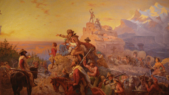
Figure 11.1 Westward the Course of Empire Takes Its Way by Emanuel Leutze
(Source: http://commons.wikimedia.org/wiki/Category:Public_domain)
From these historical events, we can see that the American social and cultural milieu of the mid-nineteenth century (like the period before it) inhibited the spread of quantification. Ordinary folks were too preoccupied with building their new land for quantification to take hold. They were not psychologically ready for such a change. In this environment, there were few mathematical inventions emanating from third-level institutions across North America—despite America’s many vibrant universities, including Yale, Harvard, the College of William and Mary, and the ten original great land-grant institutions west of the Mississippi River, including the Universities of Missouri, Nebraska, Iowa, and Wisconsin. Today, there are seventy-six land-grant universities, and the list is growing.
Hence, the sources of quantification were extant in Europe and Great Britain but not in America. That was yet to come.
In Russia, the reasons for inhibiting quantifying developments were wholly different. During the mid-nineteenth century, Russian society was still semifeudal and lagged far behind developments on the Continent. The government of the Romanov family was weak and corrupt, losing war after war, such as the Crimean War and the Russo-Japanese War. The tsars were willing to sacrifice untold thousands of soldiers (some estimates run into the millions) just to keep the wars going as their means of hanging onto power. The education system at all levels was poor or nonexistent. Russians were not allowed to travel abroad, and few of them were aware of just how backward their country was in comparison to others.
Further, not only was the Russian leadership corrupt and uncaring about their subjects, they were woefully incompetent. In one famous illustration of their shortsighted myopia, the Russian tsars were so desperate for money they sold a huge plot of their territory—Alaska—to the United States for a mere $7 million, roughly two cents per acre. Most readers probably already know that the purchase was negotiated by William Seward, President Andrew Johnson’s secretary of state, and was widely criticized in America, owing to Alaska’s remote locale and its then-unrecognized value. It was derisively called “Seward’s Folly.” Soon, however, it was recognized that it was a valuable asset and that the purchase was a good one. Russia later made overtures to the US government to buy it back, but, by then, it was too late.
An important historical event in Russia is emblematic of why the country did not advance in quantification, or in many other arenas, for that matter: the Decembrist revolt of December 26, 1825. Prior to this date, Napoleon had wanted to expand the French empire eastward, but his incursions into Russia had been met with strong resistance. In fact, the Russian troops, despite being malnourished and lacking artillery, drove Napoleon all the way back to France. He lost more than 400,000 troops in the ill-fated campaign. While this was a military victory for the Russian homeland, the incursion had unexpected consequences; namely, many thousands of Russian soldiers saw other countries for the first time and suddenly realized just how far their own country lagged behind in development.
When they returned home, these soldiers learned that their supreme ruler, Tsar Alexander I, had died. The next in line for ascension to power was Alexander’s son, Nicholas I. It was widely known among Russians that Nicholas was inept and corrupt. He was very unpopular. A group of officers and soldiers believed that the time was right for the military to take action. Not only did they want to overthrow the tsars, but they had a specific plan in mind. Here is an important part of the story that is less well known: the revolutionary leaders admired the notion of self-determination, especially for its role in America as embodied in the US Constitution. They thought it was a good model to follow and had plans to replicate its ideas in a new Russian constitution. They admiringly read Locke and Hume for their rationalism, and they knew of Jefferson’s writings and even of Hamilton and Madison’s Federalist Papers—all publications strongly influential to the spirit of a young America. They wanted to capture these ideals for Russia, too. They thought it would be a way forward—a way to end the norm of serfdom.
On that fateful December day, in what was, undoubtedly, a blizzardly cold St. Petersburg (the winter palace of the tsars), about 3,000 soldiers and officers assembled in Senate Square to make known their objections to Nicholas’s ascension. According to reports, Nicholas directed his troops to surround them, amassing many times more soldiers than there were protesters. The protesters were instructed to leave, but they refused. Then, the order came down to shoot a few of them. The protesters fired back, and then, not surprisingly, gunfire was everywhere. Being vastly outnumbered, the protesters were quickly annihilated, but the leaders were kept alive for a trial. Upon conviction, some of the leaders were executed, and others were exiled to Siberia, to the village of Chita, where they served a life sentence of hard labor. Later, the American explorer George Kennan met them while surveying in Siberia for a planned telegraph line to Chita. Apparently, he admired them in many regards, saying “Among the exiles in Chita were some of the brightest, most cultivated, most sympathetic men and women that we had met in Eastern Siberia” (Kennan 1891, 336). Figure 11.2 depicts a public trial for some of the Decembrist leaders.
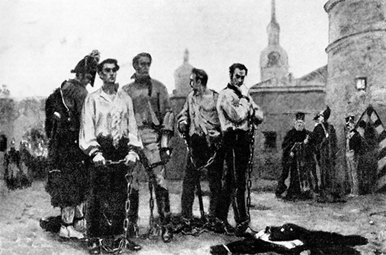
Figure 11.2 Decembrist revolt leaders at a public trial in St. Petersburg, 1826
(Source: from http://russianculture.files.wordpress.com/2010/11/x1-z5_094.jpg)
The Decembrist revolt failed that day, but it did embolden the Russian people to express dissatisfaction with the Romanovs and tsarist rule. From that day forward, unanimity in purpose grew among the Russian people as they began to flex their own brand of freedom. It took quite a while, but their sentiment eventually led to the Russian Revolution in 1917.
As you can see, the realities of life in Russia at the time left little room for intellectual pursuits such as advancements in mathematics or probability. It explains why the movement to quantification was slow there.
The reasons for negligible scholarly achievements in the Middle East and Islamic countries during the early nineteenth century were different still, yet obvious, including (1) perpetual warring among countries, tribes, and cultural and ethnic factions, and (2) a feeble academic environment at all levels. In this part of the world, war had been the norm for hundreds of years, stretching across generations. Particularly destructive were conflicts between the Ottomans (who ruled over Turkey and surrounding lands) and the Iranian Safavids (who claimed to have descended from the Islamic prophet Muhammad, although scholars doubt this). The holy war for Constantinople—from the Crusades of about 1095 to 1291 ce and lasting until the city finally fell in 1453, signaling an end of the Byzantium Empire—epitomized the clash of Islam and the West. This period in history foretells the current jihad against the West. The causes of such constant conflict are deep-seated and complex, and certainly beyond our scope to explore. (For an intimate history see Crowley 2005.) With regard to our purpose, however, this context made for a challenging environment for academics and intellectuals to contribute to worldwide scholarship. As a result, virtually no original, significant advances in statistics or probability theory emanated from this region of the world, despite it having had some mathematical innovations earlier in history.
The lack of consistent schooling in the Middle East at this time, as you can imagine, inhibited intellectual advancement and the movement to quantification by the populace as a whole. Despite being ancient in terms of culture and civilization, in the nineteenth century, these states had only primitive public education systems. Even a full century later in the twentieth century, most still had no laws for compulsory schooling, and many towns and villages had not built any schools at all, as reported in the first international survey on the topic, in the 1948 United Nations Universal Declaration of Human Rights (UDHR 1948). Even when schools were available, they were only weakly focused on teaching literacy and numeracy, giving more emphasis to instruction on local customs and religions.
At this time, the region had almost no third-level educational system at all, and the few institutions extant in the mid-nineteenth century—the American University of Beirut and Cairo University (still two of the best universities in the region)—were not on par with those on the Continent or in America, although these and other institutions have improved since then.
With colonization by European countries beginning at this time, some schooling did come, although it was mostly restricted to children of the colonizers and a few ruling elites. More commonly, though, children of these groups were sent to Europe for formal education. The vast majority of local children remained without proper instruction in reading or elementary arithmetic.
Deplorably, this deficiency continues today, although most of these countries have built schools and have finally enacted laws for compulsory education. Still, doing even this basic government service has taken more than a century after virtually all other countries. But troubles persist. A 2016 report by the United Nations Children’s Fund, or UNICEF)—updated annually as The State of the World’s Children—reports that, in 2016, almost 50 percent of children (more than 24 million) in Syria, Iraq, Iran, Yemen, Libya, and Sudan were denied education because of ongoing wars and governmental inadequacies. More than one-quarter of school buildings have serious war-related damage. They label it “a vicious cycle of disadvantage” (UNICEF 2016). It is beyond disgraceful that these governments do not provide such a basic service for all the children under their jurisdiction and for whom they are responsible.
Napoleon’s invasion of Egypt at the turn of the century did bring new markings of scholarship, then by the founding of Egyptology to study the pyramids and other historical ruins and artifacts. As a side benefit, Napoleon’s incursion slowed the recurrent looting of historical sites.
This brief description of events in the Middle East and Islamic countries during the nineteenth and early twentieth centuries conveys only a hint of the history and culture of these people and lands. However, it does provide enough context to understand some of the reasons for the paucity of scholarly accomplishment during this period and to understand why it would be slow to integrate a modern, quantification mindset among its people.
From the above, we see that, in the middle years of the nineteenth century, the journey toward quantification continued, but unevenly: heavily so on the Continent, in Great Britain, and in the Nordic countries, but more gradually in America; then, quite a bit more slowly in Russia, and more slowly still in the Middle East and Islamic countries.
Still, quantification continued, despite its uneven pace.
* * * * * *
Unexpectedly, a brilliant English engineer named Charles Babbage also contributed to bringing a mindset of quantification to ordinary people. He was considered even to be a polymath: one who is extremely gifted in many areas. But, unlike most of the others in our story, Babbage was not a statistician, nor did he make technical advances to probability theory, despite his keen interest in the field. He was a gifted mathematician, however. It is surprising he is not more widely known, especially as he held the most prestigious position in all academia: the Lucasian Professor of Mathematics at Cambridge University, from 1828 to 1839. Recall, this is also “Newton’s chair,” which was occupied in the late twentieth century by Stephen Hawking.
Still, Babbage’s role in quantification is direct and important. He is credited with inventing a machine that is ubiquitous in modern society—one that you very likely own: the digital, programmable computer. Many historians of computers consider Babbage to be the true “father of the computer” (Halacy 1970).
On learning about Babbage, one imagines that, like today’s rediscovery of Nikola Tesla (who discovered alternating current, thereby making electricity practical to use, and is the namesake of the electric car company), interest in Babbage will revive at some point. Both men were brilliant engineers, and their work is characterized by detailed plans and drawings for inventions that were either never built or only realized in practical application many years after their deaths.
And one imagines fame will also come to another remarkable individual, Ada Lovelace, whose full name was Augusta Ada Byron. She was the daughter of famed poet Lord Byron, although her parents separated shortly after her birth, and she never knew the famous poet. Ada Lovelace was an English mathematician and an associate of Charles Babbage. She wrote an early computer code for Babbage’s machine and accordingly, she has been called the first computer programmer.
Babbage was especially facile with logarithms, and he used them extensively in his early study of mechanics. But he was frustrated by a widely recognized problem of the day. Commonly used mathematics tables were replete with errors. Remember, at the time, the values in tables were calculated by hand and then recorded in columns on a piece of paper or typeset. A man of exactitude, he deliberately set out to correct the situation.
Babbage was a friend of Laplace and admired Gauss greatly, both of whom were also of astounding intellect. One imagines that if either of these mathematics geniuses were to address the problem of inaccuracies in math tables, they would look to invent an algorithm or perhaps several of them, each to address a different table. Babbage took a different route—he sought to make a mechanical computing device that allowed a formula for input and then would efficiently produce accurate values to use in any mathematics table.
True to his engineering training, he made plans and drawings to specify his ideas. He revised them continually, each time providing more and more detail and refinements. In the end, Babbage made 500 large design drawings, 1,000 sheets of mechanical notation, and 7,000 sheets of related handwritten notes. In them, he specified a large-scale calculating machine, which he called a “Difference Engine.” Later, he renamed it “Difference Engine No. 1,” to accommodate his planned refinements.
Difference Engine No. 1 was a large and complex contraption, measuring more than 6 feet in diameter and more than 15 feet tall, with a second section that extended its length by an additional 25 feet. It had thousands of parts—hundreds of them movable! He had to invent and fabricate many of the separate pieces on his own, requiring him to also invent purpose-built machine tools. Babbage’s Difference Engine No. 1 iterated number counting via a series of wheels, each of which progressed to turn the number wheel next to it. He described his contraption as one that was “eating its own tail” (Curley 2010). Babbage’s machine accomplished his intention of producing accurate numbers for mathematics tables, and he received wide acclaim for inventing it. He was particularly admired in academic circles.
He built several of the machine’s parts along the way, often displaying them in his own house, where notables of the day, including Charles Darwin and Charles Dickens, would stop by to marvel. Even just looking at its pieces caused a feeling of wonderment, as they fit together like a complex puzzle. When he activated them by turning a hand crank, levers fell in a cascade of rolling tumblers, one onto the next. There were so many cylinders, each turning onto the next, that one could watch them fall like dominos and listen to a very satisfying sound of click after click. It must have been fun to see.
Soon after inventing his calculating machine, while on a trip to Italy, Babbage learned that he had been nominated to be Lucasian Professor of Mathematics at Trinity College, Cambridge. At first, he did not want to accept the post so he could continue to work on his Difference Engine. His friends, however, prevailed upon him, and he did accept the post after all. In the meantime, he settled in London and married, and, eventually, he and his wife produced eight children. Sadly, only three of them survived to adulthood.
During this time, he and Quetelet met, but, apparently, they had a somewhat tense relationship. Quetelet was a founding member of the Statistical Society of London, which was one of the first professional organizations devoted exclusively to studying and advancing statistics. Later, a group of statisticians included Babbage to evolve the organization into the Royal Statistical Society, but he soon lost interest in the group when no one was available to keep up its administration. A planned invitation to Quetelet never came about.
Babbage continued thinking about computing machines and eventually planned Difference Engine No. 2. This one would be different from his No. 1 engine. Smaller and much more sophisticated, it could handle all sorts of computing tasks beyond just calculating numbers for tables. He envisioned Difference Engine No. 2 to be not just a better calculating device, but a programmable, analytic computing machine—an unheard-of idea. Significantly, in addition to handling numeric data, it could accommodate symbols such as letters.
Babbage’s analytical machine would have two parts, corresponding to modern computers: a central processing unit (or CPU) and a memory storage unit. Being programmable, it would read input from a set of punch cards that contained instructions for the machine’s operations, as well as original data. Some readers may already know that punch cards were used as input to computers until relatively recently, around the 1970s or so, when computer language advanced to the point wherein an operator (now, “programmer”) could type machine code directly.
I remember using punch cards with mainframe computers in the 1970s and ’80s. I even keep a stack of them from the old days, but now they are just interesting as history and no longer useful. It was also in the 1970s that ingenious youngsters like Steve Wozniak, working in his parents’ garage with his high-school friend Steve Jobs, made Apple-1, a very small computer that was easy to use. They called it a “personal computer.” Soon, they were joined by another exceptionally bright young man, Harvard dropout Bill Gates, who was a whiz at programming and marketing. He made an operating system for the personal computer that he licensed to IBM for installation on their computers (foregoing their offer to buy it outright) for a small payment for each one they sold. He used that money to found Microsoft, an early software company that started with just seven employees. Today, of course, Apple and Microsoft are two of the largest—and richest—companies in the world.
Back in the 1830s, however, true to his meticulous nature, Babbage set about making plans and drawings for Difference Engine No. 2. As before, he made hundreds of drawings and notes that described each piece in detail.
There is yet another part to the story of Babbage’s progress on Difference Engine No. 2, and this one does not relate to the machine’s technical aspects. His work was funded by the government, and officials were becoming skeptical of his ever producing anything useful. Also, he had trouble locating a suitable building to accommodate the planned monstrosity, despite its being smaller than the No. 1. The building needed to be very long, well lit, and dust-free. Eventually, the government lost confidence in Babbage’s work and, in 1842, refused to give him more money. With this unhappy development, he simply lacked the resources to build Difference Engine No. 2. Expressing frustration, he wrote, “The drawings and parts of the Engine are at length in a place of safety—I am almost worn out with disgust and annoyance at the whole affair” (Babbage 1834).
Babbage never built his Difference Engine No. 2 in full, but, in 2002, more than 150 years after he was forced to abandon his unfunded project, a group of Cambridge University students, evidently Babbage devotees, did build it. They used only the materials available to Babbage and faithfully followed his plans and drawings. When it was completed, they discovered that Babbage’s computer worked exactly as he predicted, which highlights his amazing accomplishment. Their creation is at the Science Museum in London, and a duplicate resides in California at the Computer History Museum in Silicon Valley, near Stanford University.
To see and hear this machine work is marvelously entertaining. It is truly a wonder, not only for its purpose but in the beauty of its mechanical engineering. A picture of it is given in Figure 11.3. Remember, this machine is more than 8 feet tall and 20 feet wide. Turning the hand crank requires a fair amount of force; one must stand beside the machine, which is elevated on a wooden platform. To our good fortune, a YouTube video is available for just this purpose at the referenced site (see Computer History Museum and Microsoft Research 2012). What a beautiful and graceful machine.
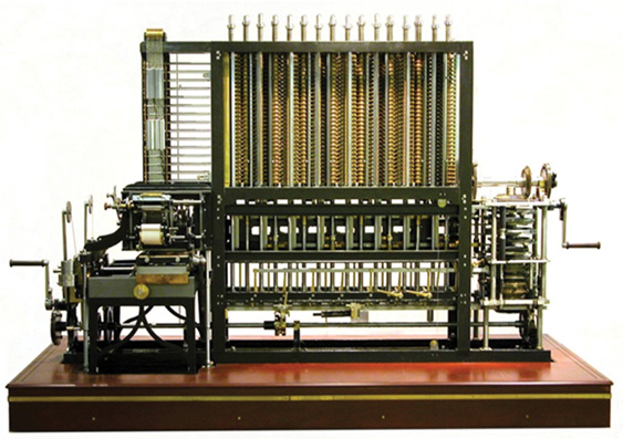
Figure 11.3 Babbage’s Difference Engine No. 2
(Source: http://commons.wikimedia.org/wiki/Category:Public_domain)
To think, Babbage’s Difference Engines—first, the behemoth No. 1 and then his plans for No. 2—were one of the first versions of a modern computer, which has spun into modern evolutions like the smartwatch and the mobile phone. Today’s “Difference Engine” weighs only a few ounces and fits on your wrist or in your pocket, yet has exponentially more computing power and storage capacity than did Babbage’s inventions. But realize they are still just programmable analytic devices with two elemental parts: a processor and a memory unit—all springing from the imagination of Charles Babbage, who worked nearly two centuries ago.
The following slight digression is an end note for those who may claim that the first true computer was ENIAC (Electronic Numerical Integrator and Computer), built in 1943 by John Mauchly and J. Presper Eckert. Their machine was the size of a small house (at 1,800 square feet), and was built with 17,500 vacuum tubes, 7,200 diodes, and miles of wire. ENIAC was different from Babbage’s mechanical Difference Engines in that it was electrical, using circuits to open and close electronic pathways for various calculations. While this was a significant innovation, it also made the machine a monstrosity to use. Whenever a new program was to be run, ENIAC required that the wires first be rerouted, a daunting task that took many hours for even a slight change. But, elementally, ENIAC drew its design from Babbage’s ideas for the computer’s two parts: a central processor and a memory unit.
* * * * * *
Earlier, we saw that both Laplace and Quetelet employed probability in research on crime and related social behaviors. Only a few years later, Siméon Denis Poisson, a pure mathematician and physicist, continued their work, but followed Laplace’s methodology over that used by Quetelet. He advanced their work by developing a particular kind of distribution useful in a specialized circumstance when there are few occurrences over an extended time period, which could be used for, say, showing the likelihood of severe earthquakes over a period of years or forecasting the number of cars that might drive through a red light at a particular intersection. These events occur, certainly, but only infrequently.
With the kinds of probability distributions we have seen thus far—binomial and Gauss’s normal distribution (the bell curve)—it is not easy to display these occasional circumstances. When illustrated in these ways, the distributions plot to a figure that is either almost flat or so heavily skewed that it is not easy to follow. The “Poisson’s distribution” fits these rare-case scenarios, and, by it, one can readily see the likelihood of occurrence for an infrequent event. In a moment, I’ll explain the Poisson distribution more fully and illustrate it with some examples, but, first, a bit about Poisson himself.
Poisson grew up near Paris in a family of modest means. His father was in the military, although he later deserted due to the poor healthcare at the time, but he saw to it that his son received a good primary education. Siméon was a very bright youngster, although not of genius level, and he was especially hard-working at his school subjects. He showed a special aptitude for mathematics. When he entered École Polytechnique in Paris, his professors (one of whom was Legendre) noticed his mathematical ability and allowed him special liberty to study the mathematics subjects of his choice. While only eighteen years old, he wrote two lengthy and notable papers, both on the calculus of finite numbers and differential equations. Legendre and Professor S. F. Lacroix (another of Poisson’s instructors) recommended that the papers be published in an important academic outlet of the day called Mémoires présentés par divers savants étrangers à l’Académie (Memoirs Presented by Various Foreign Scholars at the Academy). For a young person only two years into university, this was quite an accomplishment.
Poisson demonstrated a laudable work ethic through his life, as he eventually published many books and more than 300 technical papers, some of them so long that they were considered treatises. However, most of these publications did not offer original inventions; rather, they typically extended the work of others or provided numerous examples of applying a given theory or idea. The noted historian of statistics Stephen Stigler characterized Poisson’s work as follows:
His work in these areas (mechanics and the theory of heat) was solid but not of a class with his predecessors, Lagrange, Laplace, and Fourier. In all of this work, his role was that of a competent and insightful extender rather than that of a bold originator, and the same is true of his work in probability and its applications. (Stigler 1986, 182)
Stigler’s rather harsh assessment of Poisson is not to suggest that he was unsuccessful in his work; rather, just that he was not particularly original. Upon graduating from École Polytechnique, and with the enthusiastic support of his mentor and, by then, friend Legendre, Poisson was appointed to the faculty, filling the shoes of a vaunted professor, Jean-Baptiste Joseph Fourier. Fourier was renowned in his field at the time and is still today, and his academic chair was a prestigious one.
I digress here to mention Jean-Baptiste Fourier, even if only briefly, to convey the significance of Poisson being named his replacement. Fourier worked in theoretical physics, where he made numerous important contributions. He is best known for his Fourier transform, something which Lord Kelvin called “a mathematical poem.” This transform deals with heat transfers and vibrations, and, in it, Fourier invented a way to express how heat decomposes as a function of time into the frequencies that make it up, in the same manner in which a musical cord is heard as the frequencies of its constituent notes. The Fourier transform is so widely used in modern physics that it is a virtual necessity in the field. If Fourier had invented only this, it would still show his stature. His replacement (soon to be Poisson) would have to be someone who could carry forward the position’s reputation.
Here is one more interesting note on Fourier: he also invented a way to assess how radiation degrades Earth’s (and other planets’) atmosphere, creating what he first termed “greenhouse gases.” Even superficially, we recognize that the greenhouse effect is a part of explaining how a planet warms. He made this discovery in 1798 while accompanying Napoleon on a trip to Egypt as a scientific adviser. While there, he demonstrated how Earth is warming year by year due to greenhouses gases. This finding of global warming—made long before carbon or fossil fuels were commercially exploited and when Earth’s population was less than one billion—is regularly cited in today’s climate-change debate.
For our story, Poisson, evidently, did fill Fourier’s shoes as a professor: he gained a reputation as an excellent teacher and quickly worked through the academic ranks to full professor in 1806, at just twenty-six years old. Further, Poisson must have been an able administrator, too, because, for the next twenty-five years, he was also responsible for making academic appointments at his university, as well as for developing the curriculum. Here again, we see that he worked ceaselessly to carry out his all of his pursuits as professor and busy university administrator, as well as remaining a researcher and prodigious writer. Obviously, Poisson was a man of enormous energy and drive. Reportedly, he said, “La vie c’est le travail” (“Life is work”; Wikisource 2018).
Having gained recognition early in his career, Poisson was admitted into the prestigious Académie Royale des Sciences de l’Institut de France. There, he enjoyed a certain status. He was by then friends with several other famous members, including Laplace, Legendre, and the chemist Antoine-François Fourcroy. As a scholarly group, they held fast opinions on contemporary academic issues.
One topic of the day—the theory of light—was being increasingly scrutinized by scientists. Poisson and his Académie colleagues believed in the particle theory of light as opposed to the wave theory, a notion that was gaining acceptance in scientific circles outside of Poisson’s group. In 1818, Poisson thought he would put the debate to rest once and for all. He suggested that the Académie hold a contest in which they would offer a prize for the most persuasive essay proving one theory over the other. Poisson’s own entry argued the particle theory. He wrote a paper that did not use much mathematics or present scientific results; instead, his thesis relied on intuition. His premise was that an elemental notion of the wave theory was false. He pridefully disseminated his paper widely and was ready to receive the prize and the attendant recognition. However, it did not go well for Poisson. The judging committee was headed by the mathematician Dominique-François-Jean Arago, who conducted his own experiments—with accompanying calculations—to prove that the wave theory notions were correct after all and that Poisson’s rejection of the theory was itself faulty. Poisson was humiliated, and his reputation suffered. This stain followed him for the rest of his career. Meanwhile, Arago, who was also connected to political circles, went on to become prime minister of France in 1848.
Before exploring Poisson’s work, I pause to point out how to properly pronounce his name, since it is so often mispronounced, except of course by persons who are fluent in standard French. His name is included in his most famous contribution to measurement: the Poisson distribution. Sometimes Poisson is mispronounced as “poison.” (It is decidedly not the “Poison” distribution!) The correct pronunciation of his name is “pwa-son,” the final syllable rhyming with French “bon.” Many readers will know that poisson is the French word for “fish,” or a fish course in a meal. I imagine he would like to have had his name pronounced correctly, especially by future generations of mathematicians.
Poisson’s magnum opus was Recherches sur la probabilité des jugements en matière criminelle et en matière civile (Research on the Probability of Judgments on Matters Criminal and Civil), published originally in 1837 (Poisson and Sheĭnin 2013). In it, he extended the work of Laplace, particularly his work on jury behavior in criminal trials. One particularly vexing circumstance routinely arose for researchers working in this area: namely, how to display the relative infrequency of crime incidents for an entire population. When considered as a frequency by a binomial distribution (i.e., convicted of criminal activity: yes or no), the overwhelming indicator was no, making frequency plots for these infrequent events highly skewed and not very useful. Poisson found a way to consider such seldom-occurring events.
In statistics and probability, a seldom-occurring event is called a “rare event.” This is a circumstance that happens only once in a long while among many occurrences, such as experiencing an earthquake among many days without earthquakes, a home run among many times when batters do not hit it over the fence, or failure of a manufactured part among the many times that it performs properly. As you can imagine, plotting rare events and figuring their probability is extremely useful to research and planning. Some examples of real-world questions will help to give the idea of what is conveyed in a Poisson probability. Consider these questions:
•A traffic planner may ask: “What is the likelihood that five cars will drive through a red light at a particular intersection in a day? What about ten cars?”
•A health researcher wants to know: “What is the chance of discovering at least one coliform bacterium in a 10 cc sample of river water?”
•A hospital administrator may want to know: “What are the odds in the hospital of having five births during the hours from midnight to 6 a.m.?”
•A charitable foundation officer, making plans for next year, may ask: “What is the likelihood of reducing malaria by 10 percent over the next year in a particular country if our monetary contributions increase by 10 percent?”
•A manufacturing company executive may ask: “What is the probability of having five parts fail out of every thousand produced in a month?”
•A real estate developer may want to know: “What are the chances of selling six new houses every month in a given neighborhood?”
•A game officer may want to know: “What is the likelihood of the moose population in a given national forest doubling every five years?”
Notice several features of these scenarios: (1) they are expressed as a probability, (2) they occur relatively seldom among the many times they do not occur, and (3) the probability is within a given time frame. Time is the most common variable used in Poisson probabilities, but another scalable unit—such as a liquid measure like ounces or the pressure for gases—could be used.
Poisson considered such events as binomials: they either occur (yes) or they don’t (no), like predicting heads in a coin toss or whether a car drives through a red light. But he realized that such frequency counts (as is done in the binomial) for rare events would mean counting only a few for yes and many for no, resulting in a distribution that is so lopsided when plotted as to be unhelpful. Poisson looked at them at a much more granular level and focused on making a probability for observing an exact number (as small as zero, and typically fewer than ten) of rare events. In other words, a Poisson probability is the likelihood of observing a given number of, say, “yeses” for a rare event among many occurrences. Such a probability is a Poisson probability. Hence, a Poisson probability is much like a frequency count of a binomial, but it is expressed as a probability. There are technical differences between the binomial and the Poisson probability, but they need not concern us here.
Poisson probabilities are often plotted for several values, as in Figure 11.4, to create a Poisson distribution. Seeing the curves of a Poisson distribution also helps us to understand this special kind of probability. The figure gives three scenarios, each a Poisson distribution and shown by a different line. The horizontal axis is specified as a unit interval, which is usually time. In this figure, the numbers range from 0 to 20, which could be minutes, hours, or years. Let us continue, using the previous example of forecasting the number of cars that might drive through a red light at a particular intersection. For this, we use the unit of hours, so the baseline is zero to twenty hours.
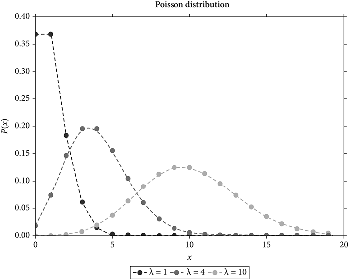
Figure 11.4 Illustrative Poisson distributions
The vertical axis (along the left side), is the probability. Theoretically, since probability goes from 0 percent to 100 percent, the scale would range from zero to one hundred. But, as is typical, the display is truncated to save space (given that, in this example, about 37 percent is the highest percentage, the scale is truncated just above it, at 40 percent). The researcher stipulates the number of occurrences for which a probability is determined. In this example, three circumstances are specified in the figure (1, 4, and 10), meaning that we want to know the likelihood of the event (a car driving through the red light) occurring just once, four times, or ten times. Then, the three Poisson distributions are calculated. Each curve represents the probability (which is read off the vertical scale) within the time frame (read as hours on the horizontal scale). For example, suppose we wish to discover the probability of one car running a red light within a five-hour period (see the left curve). Reading off the vertical scale, we see there is a less than 1 percent likelihood of this event. However, within a given five-hour interval, there a roughly 20 percent likelihood of seeing four cars run the red light (see the middle curve). For seeing ten cars run the red light in a ten-hour interval, there is about a 13 percent chance (see the right curve).
With this understanding, then, we can readily imagine that Poisson distributions are a special type of odds ratio. But they are not calculated in the same manner as the odds ratios of conditional probabilities that we saw earlier. Nevertheless, calculating Poisson probabilities and plotting the Poisson distribution are not technically difficult, although this does take us afield of our purpose. The interested reader may find any of number of Internet sites and textbooks that work through the computation. Also, obviously, there are statistical assumptions being made (about the independence of each time interval, the proportionality of disjoint time intervals, etc.), but they do not concern us here.
Poisson invented his probability calculation and attendant distribution early in his career, publishing the idea in Recherches sur la probabilité, his important work introduced earlier. But as obviously useful as the idea seems, it was not immediately picked up by mathematicians or other researchers of his day. This is surprising, as quantification as a concept was rapidly advancing at this time, and Poisson was a noted public figure. It was not until sixty years later, in 1898, that a Russian economist named Ladislaus von Bortkiewicz grew interested in the Poisson distribution and included an example using deaths by horse kicks in the Prussian cavalry in his first statistics book, which had the peculiar title Das Gesetz der kleinem Zahlen (The Law of Small Numbers; Bortkiewicz 1898).
His example was certainly meant to be serious in intent, but it was also novel and captured the attention of many individuals, giving wide exposure to the Poisson distribution. Over the years, this example has become famous for illustrating the Poisson distribution—it is referred to as “Poisson’s horse kick data” or similar.
Bortkiewicz collected the rather unusual statistic of annual deaths in the Prussian cavalry by horse kick. He gathered the values for a twenty-year period (from 1875 to 1894) for ten army corps, yielding 200 total observations. He compared the actual number of deaths (122 out of 200 points of data) to that predicted by Poisson probability, thereby demonstrating the accuracy of Poisson’s method. His results are shown in Table 11.1.
Table 11.1 Annual deaths from horse kicks in the Prussian army (1875–94)
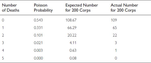
In the table, note there are four columns: number of deaths, Poisson probability, expected number for 200 corps, and actual number for 200 corps. The rows show values for the number of deaths in a year: 0 to 5. The first row is information about 0 deaths per year in the 200 total observations: the Poisson probability of 0.543 yields the Poisson estimate of 108.67 years (out of 200) without any deaths, perfectly accurate to the observed 109 years with 0 deaths. For an estimate of 1 death per year, the probability estimate is 0.331, yielding 66.29 years when there was only a single death. This estimate is compared with the actual 65 years in which just one death occurred. Again, the Poisson probability estimate is very close, as it is for each of the other rows of probabilities. He thereby demonstrated the accuracy of Poisson probabilities. For whatever reason, Bortkiewicz’s illustration almost immediately became well known and led many others to adopt Poisson probabilities as a useful methodology.
A popular party game today uses Poisson probabilities in its solution, although it is doubtful that any of the guests realize it. The point of the game is to guess the likelihood that any two players have the same birthday. The guests simply state their birthdate, and the fun is to discover whether two share the same date. It turns out that, with only about two dozen guests, there is a nearly 50 percent chance that at least two share a birthdate, although, obviously, an individual’s birthday could fall on any of 365 days. The probability calculations are relatively simple but a bit tedious to explain; they can be found on many Internet sites, including one sponsored by the University of Massachusetts (see University of Massachusetts 2017).
* * * * * *
Like Laplace, Poisson believed in the universal applicability of probability, as he stated many times in Recherches sur la probabilité. As such, he was fascinated with how numbers operate and explored not only the binomial theorem but also other related number theorems. Recall from Chapter 4 that we explored three foundational number theorems: the binomial theorem, the law of large numbers, and the central limit theorem.
In fact, Poisson gave a name to Bernoulli’s theorem (originally Theorema aureum), calling it “the law of large numbers,” the name we use today. He extended it to the circumstance wherein there is not always a fifty–fifty chance for each of two outcomes and there can be an unequal success probability across a number of trials. This was called “Poisson’s law of large numbers.” It is not nearly as well known as Bernoulli’s law because the instances in which it arises are fewer.
But Poisson did introduce a notion that is common: namely, that of a random variable. As we saw earlier in Chapter 9, in probability theory, a “random variable” is one that must assume a discrete number, such as 0, 1, 2, or 577. Some examples of “discrete random variables” are the number of children in a given family, and the number of minutes someone waits in a line at a grocery store. It is random because the outcome is completely unknown: choose another family and the number of children may or may not be different, or take another trip to the store and the time you wait in line may be completely different. Another type of random variable is the “continuous random variable,” which is a number along a scale, such as height or a test score.
In exploring the central limit theorem, Poisson provided a calculus proof to it that had not been given by Laplace when he invented the theorem some years earlier. Laplace had devised the theorem but had relied upon intuition and common logic as his rationale. The final proof for this foundational notion, however, did not come until later when Baron Augustin-Louis Cauchy, a French mathematician and physicist and contemporary of Poisson, proffered a rigorous calculus proof for the central limit theorem. Later still, in the twentieth century, a group from Russia, called the St. Petersburg Mathematics School, validated Cauchy’s work, which is now accepted as definitive.
Cauchy made a related mathematical invention, too, that is a demanding application of Poisson’s probability distribution and is itself a continuous probability distribution, although its application is primarily in physics rather than in probability and statistics. This mathematical framework is called the “Cauchy distribution,” but, in physics, it is also known as the “Cauchy–Lorentz distribution” or sometimes just the “Lorentz distribution,” after the mathematician Hendrik Lorentz.
All of this rigorous work has special meaning to the overall flow of quantitative thinking, too, because it signals a period in the development of probability theory in which precise, rigorous, and thorough proofs are required before developments would be widely accepted. By this new demanding standard of the mid-nineteenth century, probability theory was given credence as a rigorous and independent discipline within mathematics. As one historian of mathematics notes,
The mid-nineteenth century saw a new era in mathematics with the introduction of rigor in analysis, spearheaded mainly by Cauchy and then followed by many others. Among other things, rigor meant that every mathematical concept used had to be explicitly defined in terms of known concepts and that all assumptions in a mathematical proof had to be made explicit. Rigor also meant that mathematical ideas were based on precise and exact concepts, rather than on intuition. (Gorroochurn 2016a, 139)
For our story, from the early to mid-nineteenth century social and cultural events described in the opening pages of this chapter to the closing notes on the demands for rigor and exactitude in probability, people’s thinking has been moving ever closer to quantification. In routine areas of life for ordinary folks (that is, nonmathematicians and nonacademics), there is an induction of quantification.