CHAPTER 13
Galton’s protégé and biographer, Karl Pearson, was one of the first to chronicle the history of statistics. In doing so, he made the following observation: “It is impossible to understand a man’s work unless you understand something of the environment. And his environment means the state of affairs, social and political, of his own age” (Pearson and Pearson 1978, 360). This statement is much to the point of this book, too, for throughout it, I have tried to provide a meaningful context for the mathematical achievements that led to our quantified worldview.
Since opening our story in Chapter 1, I have maintained that the astounding technical, quantifying inventions, discoveries, and advancements we have witnessed were made because they could happen, in deference to a period in history whose events encouraged scholarship. Pearson made his remark in a book whose full title gives even more detail to this notion: The History of Statistics in the 17th and 18th Centuries against the Changing Background of Intellectual, Scientific, and Religious Thought (1978).
In parallel fashion to Pearson’s recounting of the history of statistics in earlier centuries by also chronicling contemporaneous historical events (“background of intellectual, scientific, and religious thought”), we now view the phenomenon of quantification in the nineteenth century through the context of the events of that period. We saw at the end of Chapter 12 that, with Galton’s invention of psychometrics, quantification was finally spreading to America. Accordingly, we now explore the what, how, and why of this expansion of quantification by looking first at the societal events in that country.
Two events—even beyond the Western expansion described in Chapter 12—define this century in America: the Industrial Revolution and the Civil War. Because societal influences are not cleanly bounded for either of them (despite the Civil War’s battlefield dates of April 12, 1861, to May 9, 1865, by proclamation), it is not possible to precisely tie a particular advance in the quantitative fields of mathematics or probability to a specific happening in either era. Nonetheless, there is enormous convergence of technical developments in probability and statistics with these historical periods, and this is what I describe herein.
Historians often cite the invention of the cotton gin as instrumental to the beginnings of both the Industrial Revolution and the Civil War. This machine was invented by Eli Whitney in the late eighteenth century and finally patented (after a number of delays) in 1808. Whitney’s invention bears on the Industrial Revolution in two important ways. The first is its impact on the economy of the Antebellum South of the United States (covering the period from the late eighteenth century to 1861, the start of the Civil War), and second is the machine itself, for its innovation of having interchangeable parts.
Prior to Whitney’s machine, cotton could only be processed in small amounts. Before it can be spun into cloth, the seeds must be removed from the cotton bolls. When done manually, the task is slow and tedious to the extreme. Even more important, it is punishing on a worker’s hands and back. The cotton gin transformed the production of cotton by doing the job mechanically, and that made all the difference. Separating seeds from bolls by a machine was many times faster than before and was not so physically grueling on the operator. Thus, with the cotton gin, huge quantities of the crop could be processed efficiently. From the Antebellum South, the soft, clean bolls were sent north to awaiting textile mills where the cotton was spun into cloth and garments made.
At first blush, this may appear to be a wonderful advance (and mechanically, it was), but there is another step in producing cotton that the cotton gin did not change: picking it in the fields. At the time of Whitney’s invention, slavery was legal in Southern states, and land owners relied on enslaved Africans for plentiful, cheap labor. With vastly increased crop production, Southern economies soared. Some powerful landowners built plantations (some of which encompassed many thousands of acres) and built for themselves gigantic, ostentatious houses. But the backbreaking work of picking the cotton continued as before, only now with many more slaves.
At the same time, several states were seeking to join the Union, and whether they should allow slavery was hotly debated as an issue of state’s rights. Initially, the public disagreement was less focused on the moral issue of owning slaves and more on whether to count them as citizens who should be taxed (with the levy to be paid by their owners). Soon, however, in addition to states’ rights, the argument broadened in scope to include the ethics of slave ownership. As the northern states demanded full taxation (and because slavery featured prominent in the South’s position), the South saw secession as the answer. As readers likely know, the period included the notorious “Missouri compromise” and a number of important court cases (e.g., Dred Scott v. Sandford).
There are, of course, libraries full of books and videos telling this involved story more completely. The classic work is Shelby Foote’s three-volume masterpiece, The Civil War: A Narrative (Foote 1986). Foote’s wonderful work is also the basis for much of Ken Burns’s engaging video series The Civil War (Burns et al. 2004). Experiencing both Foote’s book and Burns’s video is time well spent (Foote is interviewed extensively in the video series).
We can see, then, that the cotton gin was instrumental in contributing to events that eventually led to the American Civil War. Nearly everyone was either personally or very closely affected by the experiences of this era in American history. In terms of our current inquiry, the period slowed progress toward quantification in the same manner that most Europeans had been constrained in thought by the Napoleonic era—in both times, people were fully occupied with the strains of daily existence. But, obviously, any period in history as complex as this had mixed influences, and some of them were supportive of the path to quantification, although clearly these countervailing influences were not nearly so strong as to negate the effects of the war on the public’s mindset. Nonetheless, two simple examples will illustrate this point: the 1860 United States Census and, from sports, the even earlier formation of the National Baseball League (in 1857), initially the National Association of Base Ball Players (NABBP).
The United States Census of 1860 was particularly important because the issue of states’ rights was front and center in public debate. Due to the period’s severe tensions, the census was abbreviated, but it still tabulated a 35 percent increase in population over the previous census in 1850, from 23 million to nearly 34 million. Relevant to the heated public debate, this number included more than three million individuals listed as slaves. Since each family unit was personally contacted for the census, it brought counting and the notion of aggregating data into direct contact with millions of ordinary folks. Figure 13.1 shows a page from that census.
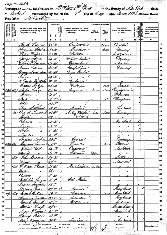
Figure 13.1 Page from the 1860 United States Census
(Source: http://commons.wikimedia.org/wiki/Category:Public_domain)
Another fact of the day that brought numeracy to a vast population—and thereby fostered quantification—is seen in the game of baseball. Immediately upon the official close of the Civil War in 1865, baseball was already gaining a following: NABBP league games had been played since 1857. It happily and easily became the national pastime. Its popularity at that time has never been equaled by any other sport.
A student of the game and one of the best writers to capture its deep meaning to Americans, George Will, claims that, in post-Civil War America, baseball was a calming influence, helping to heal the wounds of a divided nation (see Will 1990, 295). He makes this observation in one of the best books on the sport ever written: Men at Work: The Craft of Baseball, although it is now a bit dated (Will 1990). As is widely realized, since the first league baseball game was played, the sport has had an obsession with keeping game statistics on everything imaginable, from runs, hits, and errors to (seemingly) what occurred during which phase of the moon. Even today, there are sponsored contests that draw a huge following, matching contestants on their knowledge of arcane baseball statistics. Also, here is an interesting, relevant side note: the official site of the sport states that the game’s inventor, Abner Doubleday, made up the initial set of rules in 1839 and later went on to become a Civil War hero.
Also in this era, and despite the end to Civil War fighting, the so-called Indian Wars continued, forcibly (and shamefully) relocating Native Americans to reservations and sometimes even breaking agreements in order to force them onto less desirable lands. One battle of the Great Sioux War of 1876—infamous in song and legend as “Custer’s Last Stand”—took place over two days (on June 25 and 26) along the Little Bighorn River on the Crow Indian Reservation in southeastern Montana Territory. A 36-year-old Army general with personal ambition, George Custer, disobeyed his orders to hold fast to his locale on the edge of the prairie and instead led his troops onto native lands, with the intention of forcing the people there onto a reservation. The famous eponymous battle ensued. When the action ended, all of General Custer’s 600 troops lay dead in the prairie grass, leaving a single horse named Comanche as the only Army survivor. About 180 Crow warriors had been killed, too. This was a sad and shameful day in American history.
Will puts this event and the game of baseball in a perspective that is both enlightening and unexpected. He said, “The day Custer lost at the Little Bighorn, the Chicago White Sox beat the Cincinnati Red Legs, 3–2” (Will 1990, 293). While Custer’s loss is well known, there is less awareness that many in his regiment were recruited from baseball teams, with them often saying they were eager to get back to playing the game as soon as the battle ended. This was a remarkable juxtaposition of events.
More than any other sport in America, baseball, with its immersion in game statistics, is emblematic of quantification, since its invention to today.
* * * * * *
Eli Whitney’s impact on the Industrial Revolution and the Civil War era extended beyond simply the cotton gin, as revolutionary as that invention was. He also designed an “in-line process” for making muskets in quantity by manufacturing and assembling them in pieces at stations. For this process, Whitney’s workers were stationed in a line where each one would add a specific part to the gun and pass it on to the next worker. Prior to this manufacturing innovation, guns were made one at a time by a single worker, a process which took a lot longer. Using Whitney’s manufacturing method, these long guns became cheap to produce. Due to this innovation, Whitney is considered the “father of mass production.”
Ever the clever inventor, Whitney also engineered the guns to have interchangeable parts, another important first. The advantage of interchangeable parts is that the guns could be repaired in the field by infantrymen. Thanks to his rapid in-line process of mass production and the feature of interchangeable parts, Whitney’s muskets were clearly attractive to large buyers. Whitney demonstrated the steps in his mass-production process before a session of the US Congress, where he assembled a gun from its separable parts in just a few minutes. At the conclusion of his presentation, he was immediately awarded a huge contract for many thousands of muskets.
Some historians have noted the supreme irony that this one man had so much to do with both sides of the Civil War: first, by advancing the South’s economy through his cotton gin and, second, by producing vast quantities of guns for the North’s military war effort, helping it win.
Plainly, the Industrial Revolution on both sides of the Atlantic was one of the most momentous periods in all of human history. Nearly everyone in the Western world was directly affected by it, many to a life-altering degree. Often, historians note that even more significant than the inventions and innovations of the period was the fact that the Industrial Revolution brought forth tremendous and sustained progress in the standard of living for most people. Folks of meager means and only ordinary opportunity were better off almost overnight, or certainly within the span of one generation, living lives of much more convenience. They had better healthcare, superior education, and, for a time anyway, there was less direct impact on daily life from national wars and conflicts.
For context, remember, this improvement is judged by the living standards then, sans “presentism”—one need only check Dickens to be reminded of daily hardships in working conditions brought on by the Industrial Revolution, too. Figure 13.2 illustrates some of the infamous circumstances wherein men and women—often while still in their youth—toiled in tedious and frequently dangerous conditions.
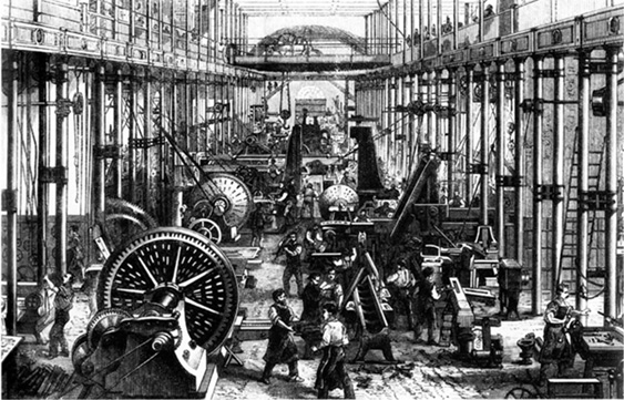
Figure 13.2 Workers at machine works company during the Industrial Revolution
(Source: http://commons.wikimedia.org/wiki/Category:Public_domain)
Pertinent adjectives to describe the Industrial Revolution spring forth in such volume that the words themselves could fill a treatise: imaginative, inventive, hard-working, creative, visionary, inspired, resourceful, ingenious—and I must mention two obvious descriptors: industrious and revolutionary. There is considerable debate among historians and sociologists about what years encompass this period and which inventions and innovations to include in its discussion. I follow several historians who cite the invention of the steam-powered railway as the Industrial Revolution’s start. By this, it began in England in the early years of the nineteenth century when queues were long, with folks waiting their turn to ride the new Stockton and Darlington Railway in 1825 (see Chapter 12, Figure 12.1). Some folks climbed on board just for the novelty of this newfound freedom, but more were discovering it to be a means to expand their businesses and other enterprises.
Ocean liners, too, were being powered by steam, and transatlantic travel was becoming more practicable—although, of course, beyond the reach of most people. Inventions, discoveries, and innovations of the same ingenuity as steam-powered engines were happening so fast that people could scarcely keep track, much less absorb their impact. Nonetheless, everyone knew about the newly harnessed power source and other inventions, and it set forth a spirit of “I can do that, too.” Worldwide, there was a new sense of possibility. In America especially, the production of steel at huge steel plants (mostly located in the Northeast) and the drilling of oil in vast oil fields in Texas, Oklahoma, and throughout the West, came to dominate industry. The textile industry, spurred on by the invention of the cotton spinning machines, was flourishing, first in Great Britain but soon all along America’s East Coast.
These formative years in American history are chronicled in a marvelously informative book titled What Hath God Wrought: The Transformation of America, 1815–1848 (Howe 2007). (Note: this is Volume 5 in the comprehensive series The Oxford History of the United States and, in 2008, won the Pulitzer Prize for History.)
As one might expect, numeracy and quantification were integral to much of this period. Suddenly, nearly every new thing was described in numerical terms: how big, how high, and how powerful. Technical words like “watts,” “voltage,” and “force” came into ordinary parlance. I imagine that, before such terms became the most economical and accurate way to describe the next new invention or innovation, they were not so popularly used. Now, though, people were progressively realizing that a numerical point of view was growing in influence on their daily lives—quantification was advancing.
Even more fundamentally, the sense of self seemed primed by the times to transform so as to keep apace of the quantifying events. Indeed, the relationship between mathematical inventions and the times in which they were done is almost symbiotic: people changed their lives and way of thinking because of the times—and simultaneously, many inventions and innovations that constituted the Industrial Revolution were themselves possible only because of the new mathematical discoveries.
Or, from the perspective of quantification, the people who pioneered these mathematical and probability ideas gave possibility to the inventions of the Industrial Revolution in the first place, which then fostered for us a transformed view of the world and our place in it. The concept that mathematical advances occurred because they could, which I have mentioned so many times before, is clearly evidenced here.
As everyone knows, during this period, not all inventions were mechanical; a plethora of technological inventions sprang up, too. Some were life altering in their impact. One such invention can be traced to an exact date: on March 26, 1876, newspaper headlines printed in large type the news that Alexander Graham Bell had intoned into a cone-shaped microphone, with his voice crackling, these unassuming but now-famous words to his assistant in the next room: “Mr. Watson, come here. I want to see you.” He had invented the telephone. With it, life for nearly everyone—rich and poor—was changed.
Yet another influential piece of machinery that was important to the Industrial Revolution was the sewing machine. Although various machines used for sewing had been around for a long time, the modern sewing machine really took off for popular use around 1851, when Isaac Merritt Singer added a foot pedal and applied for a patent. However, it seems a rival named Howe had already invented such a machine—he won a legal judgment against Singer, wherein Singer would pay Howe a royalty of $1.10 for each sewing machine sold. Singer’s machine was wildly popular, as ordinary folks could now sew and repair their own clothes in a fraction of the time it took to do by hand. Singer also copied Whitney’s idea of having interchangeable parts, making the machine simple to repair, sometimes even at home. His sewing machine came to symbolize modernity and played an important role in the Industrial Revolution.
Isaac Singer was an ambitious entrepreneur. After working on his sewing machine, he devised an innovative sales strategy: he added a sales force of nattily dressed individuals who went door to door selling the sewing machine to middle-class homes. And, to make the purchase more attractive, Singer (together with a lawyer named Edward Clark) devised a “hire-purchase arrangement” by which people would immediately take possession of the machine and then make payments over time—the first installment plan. These innovations were quickly adopted by others and became central to the progress of the times.
Following Karl Pearson’s observation (given in the opening lines of this chapter) that an awareness of the times is a prerequisite to understanding your work, we are now prepared to discuss the next significant quantitative development: Pearson’s own coefficient of correlation.
* * * * * *
In 1892, Karl Pearson published a book that changed the world of scientific research: The Grammar of Science (Pearson (1892) 2004). For a generation, it was virtually required reading for anyone engaged in scholarly work, almost regardless of the discipline. Einstein recommended it as the first book to read among his friends at his book discussion group Akademie Olympia (“Olympia Academy”). The title is itself telling of its comprehensive scope and unconventional approach. In it, Pearson describes the laws of modern science, both stating how they were applied (in his time) and then setting a standard for researchers that previously had not been well developed.
On the title page, he gives his book a motto that has become famous to scientists: “Statistics is the Grammar of Science.” He elaborates the motto’s meaning by emphasizing to scientists the importance of employing creative imagination rather than mere fact gathering, while at the same time remaining objective and dispassionate in following a careful methodology. In the preface (in quotes taken from its second edition, the best known today), he says,
There are periods in the growth of science when it is well to turn our attention from its imposing superstructure and to carefully examine its foundations. The present book is primarily intended as a criticism of the fundamental concepts of modern science, and as such finds its justification in the motto [Statistics is the Grammar of Science] placed upon its title-page. (Pearson 1900b, ix)
As is apparent, Pearson intends no less than to upend scientific research, placing empiricism at its center while simultaneously encouraging scholars to exercise care for objectivity and dispassion in their work. Elaborating this point, he adds:
The classification of facts and the formation of absolute judgments upon the basis of this classification—judgments independent of the idiosyncrasies of the individual mind—essentially sum up the aim and method of modern science. The scientific man has above all things to strive at self-elimination in his judgments, to provide an argument which is as true for each individual mind as for his own. (Pearson 1900b, 6)
And, in summary,
It [science] claims that the whole range of phenomena, mental as well as physical—the entire universe—is its field. It asserts that the scientific method is the sole gateway to the whole region of knowledge. (Pearson 1900b, 24)
Further, and in an innovative fashion, he made an assertion that shocked the world of researchers, declaring “all science is description and not explanation” (Pearson 1900b, vii). Clearly such words were sorely needed at the time, for as we saw in Chapter 12, when Galton warned that his description of a correlational relationship did not ipso facto mean causation, researchers were often careless about interpreting their findings.
Pearson’s approach to scholarship and definition of a philosophy of science has shaped much of scientific research from the time of the book’s publication to today. Surprisingly (and regrettably), though, apart from intellectual circles, his book is scarcely known. Today, although most scholars are attentive to protocols for methodology in their work, it is indeed unfortunate that few of them are aware of the origin of their rules.
From even this brief introduction to The Grammar of Science, it is easily seen that the work is both philosophy of science and technical treatise. As a work of philosophy, Pearson opens the book with thoughts that suggest a quantified worldview—one that would “profoundly modify our theory of life”—is needed to appreciate “so revolutionary a change” of recent scientific advancements. He begins the book:
Within the past 40 years, so revolutionary a change has taken place in our appreciation of the essential facts in the growth of human society that it has become necessary not only to rewrite history, but to profoundly modify our theory of life and gradually, but nonetheless certainly, to adapt our conduct to the novel theory. (Pearson 1900b, 1)
In this exposition, Pearson sees the world of science divided in two: the philosophical and the technical—but he resolutely believes they should be unified. To this end, while imploring the careful researcher to follow rules of scientific discipline, he coaches future researchers to be concerned with their humanity as well: “Directly or indirectly, the individual citizen has to find some reply to the innumerable social and educational problems of the day” (Pearson 1900b, 5). Here, he goes beyond Laplace, Quetelet, or even Galton, who each sought to bring sociology into their expertise. To Pearson, scientific research is qualitatively different; it is but an avenue to social consciousness—they are one and the same. Quantitative work and social ethics are “much the same character,” in that they identify and define ordinary people going about daily life:
Geometry might almost be termed a branch of statistics, and the definition of the circle has much the same character as that of Quetelet’s l’homme moyen [average man]. (Pearson 1900b, 12, note 1)
Having established form and context for scientific research, Pearson then turns his book to the technical side of his work. In this section, filling nearly half of the book, he covers a wealth of technical topics. His thoughts include a critique and extension of Newton’s original laws of motion and delve into conjecture on the space–time continuum. Perhaps most famously of all, he writes early notes on the physics of relativity, anticipating Einstein’s theory of relativity (notes which Einstein acknowledges as his inspiration; we’ll examine them briefly in Chapter 16). His chapter headings give a flavor of this section of the book. They include “Space and Time,” “The Geometry of Motion,” “Matter,” “The Laws of Motion,” and “Modern Physical Ideas.” A drawing of his notes for the book is displayed in Figure 13.3.
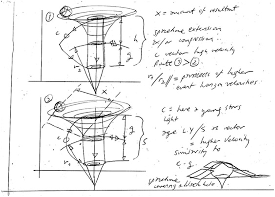
Figure 13.3 Karl Pearson’s notes for The Grammar of Science.
(Source: from http://benabb.files.wordpress.com/2010/05/img_0081.jpg, accessed August 21, 2018.)
For persons with a bent for more exploration of Pearson’s concepts, I recommend it. It is wonderful reading, with nugget after nugget of insight, all composed in an engaging style (see Pearson 1900b). Clearly, The Grammar of Science is a brilliant work of scholarship, one with many firsts. By his book and its clever motto, Pearson is sometimes credited with having invented mathematical statistics as a distinct discipline, although just as often that title is given to others.
To our purpose, the author’s words reinforce quantification more directly than any scholarly text we have seen thus far. Hence, it moves quantification significantly forward.
* * * * * *
In an especially important spark of genius, Karl Pearson developed a mathematical coefficient that made the Galton’s correlation truly statistical, now a concept with a derived proof and an empirical interpretation. Pearson did this by borrowing an idea from physics—a particular expression of a numerical scale called “moments”—and applying it to a normal distribution. “Moment” has a special definition in physics in a sine wave and some other mathematical applications, but, for our purpose, we may think of them as standard deviations: each moment represents one standard deviation, plus or minus.
Pearson’s addition of a mathematical structure to Galton’s correlation has given rise to a formal name for the statistic: the “Pearson product–moment correlation coefficient.” The name itself is more thoroughly descriptive than is common for statistical terms: it is honorary to Pearson, expressive of the relationship’s quantitative structure, and broadly hints at its calculation by multiplying the moments (i.e., standard deviations) of a distribution. The final word, “coefficient,” is essential in its proper interpretation, for it points directly to the degree of association or influence between the included variables.
Pearson used the letter r to denote his coefficient (mathematics readers will realize that the Greek letter ρ is used in some technical contexts when the statistic is applied to a population of values and not just the sample statistics). Familiar examples of r are displayed in Figure 13.4.
Figure 13.4 Pearson product moment correlation coefficient
Pearson laid out his coefficient in his famous book and expounded upon it much further in a number of follow-up papers (e.g., Pearson 1905, 1907). In these, he extended his account to include relevant considerations such as issues dealing with the size of the sample, realizing what happens when the variables are themselves skewed, or the circumstance of accommodating more than two variables.
He then built upon these concepts to introduce many other statistical terms, such as “skewness,” “kurtosis,” and “goodness of fit.” (This last term, particularly, is notable, and I will describe it momentarily.) He was the first to use the term “standard deviation,” and he formally introduced the “contingency table,” now a routine way of comparing frequency counts between categories. For example, a 2 × 2 contingency table has four cells with a dichotomy for each of two variables, as when, say, biological sex (male and female) is compared with incidents of a heart attack (yes and no). By themselves, these ideas of Pearson’s have led many others to develop still more procedures and statistical tests, some of which I’ll address in later chapters.
Pearson’s legacy is all the more remarkable when you consider that he was not formally trained in statistics, although he did have a mathematical education. Knowing what we know now about him, it is not surprising that he regularly read some of the great philosophers, such as Berkeley, Locke, Kant, and Spinoza. Although he did not write philosophy as such, it is obvious this education influenced his work in statistics and probability. We already saw this in his Grammar, and, throughout his mathematical writings, he routinely cited philosophical ideas.
* * * * * *
Given that Pearson was a protégé of Galton and an admirer of Darwin, it is not surprising that almost everything Pearson did stemmed directly from these two predecessors. Most famously, he followed them in biometrical studies, especially as they were used in personal identification, such as with physical characteristics. From early in his career, he had been interested in their findings on heredity, and, accordingly, he produced several works on eugenics, looking at such things as immigration and criminal background as variables in sundry heritability studies.
Although Galton and Pearson were friends and each admired the other’s work, they did not produce much scholarship together. But, near the end of Galton’s life, Pearson wanted to initiate an academic journal devoted exclusively to advancing theoretical statistics. So he, along with Weldon (mentioned earlier as one who cautioned against misinterpreting correlational relationships), asked Galton to join the effort. Galton happily agreed, although his role was mostly honorary. Together, in 1901, these three academics founded Biometrika. Since its establishment, Biometrika has been one of the leading journals of mathematical scholarship, near the very top even today. The articles present only the most serious and noteworthy ideas, and to have work published in the journal is a feather in any academician’s cap. For its nearly 120 years of existence, it has been published by Oxford University Press.
Pearson originally called the journal Biometrica (spelled with a c) to reflect biometric studies, but another colleague, Francis Edgeworth, changed the journal’s name to be spelled with a k to indicate a broader scope of interest.
Edgeworth was a notable scholar in economics, and he introduced the so-called Edgeworth box, a graphical representation of how economic resources are distributed. Today, in virtually all courses and texts on introductory economics, the Edgeworth box is standard fare for study. Edgeworth himself was an interesting fellow. Evidently, he was born into a wealthy Anglo-Irish family—his education was entirely by private tutors, and he never attended school. Later, however, he attended Trinity College, Dublin, the prestigious Irish university.
Returning to Pearson, one work in particular showed the influence of both Galton and Darwin. At the time of its publication, it received immediate attention from his peers and has had lasting impact, even to today. The two-volume work is titled The Chances of Death and Other Studies in Evolution (Pearson 1897). Its opening pages of the second volume are most unusual. While proposing to discuss his studies involving lifespan and evolution, he recites medieval notions of death and reproduces several woodcuts from the fifteenth-century artwork called The Dance of Death, by Hans Holbein the Younger. These strange woodcuts show skeletons in contorted positions and caricatures of persons with emaciated bodies. Pearson discourses on these macabre woodcuts as though he is reviewing previous literature to set the stage for his own work. Bizarre! Fortunately, he moves past this to more conventional scholarship wherein he presents several ideas on heritability.
The book’s influence arises from one idea in particular that has become quite famous. He introduces the notion of the “chi-square goodness of fit test.” It is commonly referred to as “Pearson’s chi-square.” This simple but effective statistical test is routine in research today. There is scarcely a beginning statistics textbook or other introductory material that does not mention Pearson’s chi-square statistic and his goodness of fit. In fact, to the degree that an early student of statistics or a beginning researcher may be aware of the name Pearson, it is probably thanks to this statistical test.
Pearson, following his earlier specification of significance levels for a correlation, set out to devise a way to determine whether a distribution of sampled data was close to or far from a normal distribution. The idea is perhaps easiest seen through example: suppose you collect data on the incidence and severity of crime in a neighborhood and want to determine whether the levels observed from that one sample are close to what could be expected if the same data was collected across all neighborhoods (considered the population). To state this in statistical terms, as a researcher would, the question becomes “Is the sample data similar to the population data?” Pearson’s chi-square goodness of fit test applies to such binomial data. To take another example, suppose you flipped a coin many times to see whether the observed results followed a hypothetical binomial distribution for the population. Recall from earlier discussion the three theorems of numbers that are relevant here: the binomial, the law of large numbers, and the central limit theory. Pearson’s test specifies significance levels for determining the closeness of sample data to these theorems; namely, goodness of fit. This is one of the first such statistical tests of difference.
To create his statistical test, Pearson needed to devise a way to gauge the distance of observed data from the theoretical population. His method for doing this was quite clever and insightful with regard to the three theorems, while at the same time remaining simple and direct. He set out to exactly specify a population for binomial values, meaning he needed enough data for it to be considered not just a very large sample but the population of values itself (which, of course, is very, very large—even theoretically infinite).
To collect such data, he used many samples of coin flips. In fact, he needed enough sample coin flips to aggregate to what could be taken for a population of all possible coin flips. Initially, he flipped a coin 2,400 times. Apparently, Pearson tired at this task, because he asked a student of his (!) to continue collecting data until he had an additional 8,178 samples. He then added even more data from outcomes of Monte Carlo roulette tables. Finally, with sufficient data in hand, he compared given samples to his “population data” and looked at the errors (he first used the term “deviations,” and then “standard deviations”).
He amassed the data in a set of response matrices. From these, he devised significance levels to identify the relative closeness of any given sample to the population. In other words, if the three basic theorems of numbers are correct, what is the probability that any sample data fit them? From this was derived Pearson’s chi-square goodness of fit test. Figure 13.5 shows Pearson’s actual distributions.
Figure 13.5 Pearson’s distributions for assessing normality assumptions
(Source: from K. Pearson, The Chances of Death and Other Studies in Evolution)
In 1900, only a few years after mentioning his method in The Chances of Death, Pearson expounded on it in an article that is now famous and is considered to be the formal introduction of his goodness of fit test. The article certainly has one of the longest titles in history, one that nearly explains the whole thing: “On the Criterion that a Given System of Deviations from the Probable in the Case of a Correlated System of Variables Is Such that It Can Be Reasonably Supposed to Have Arisen from Random Sampling” (Pearson 1900a). It is a bit surprising that the journal’s editor would allow such a drawn-out title for an article. Maybe Pearson’s academic stature held the same sway over the editor as it had earlier over his dutiful, coin-flipping student. Regardless, Pearson’s chi-square goodness of fit test is one of the most popularly used inferential statistics, then and now.
* * * * * *
As we have seen several times before, however, discoveries and inventions, both physical pieces of machinery and technical advances in mathematics, rarely happen cleanly. Nearly all have direct antecedents or have been discovered or invented elsewhere. Such is the case with the chi-square statistic. In 1876, a few years before Pearson’s publication, a German professor of mathematics at the RWTH Aachen University (a leading technical university) and innovator in geodesy named Friedrich Helmert, published a nearly identical (and slightly more sophisticated) procedure for comparing a sample’s distribution to that of a normal distribution. Hence, it seems that Helmert may actually have invented the chi-square first.
Even at the time, Helmert’s invention did not go unnoticed, as several contemporaneous statistics textbooks describe Helmert’s chi-square distribution. The context seems to have been that Helmert’s work, and that of surrounding texts, was neither translated out of old German nor widely distributed. It seems, then, that both Pearson and Helmert can lay legitimate claim to invention of the chi-square statistic. This is another instance of simultaneous and independent progress in probability and statistics.
To our modern benefit, Helmert, a fine mathematician, has not been forgotten. Together with our mathematics giant, Gauss, Helmert published a textbook on least squares that enjoyed wide acclaim. Moreover, today Helmert is remembered for a particular kind of statistical contrast. In statistical contrasts, a variable with several categories—called “levels”—is considered. For example, suppose “income” is the variable of interest and there are, say, five levels, from lowest to highest. Several combinations are possible for comparing the levels. For instance, each income category (i.e., level) can be contrasted with some reference, which is typically either the highest or the lowest income category.
With the “Helmert contrast,” each level of the income variable is compared with the mean of the subsequent levels. That is, the lowest income level is compared with the mean of the higher four levels, the second lowest income level is compared with the mean of the higher three levels, and so forth. In a “reverse Helmert contrast,” each level of the variable is compared with the mean of the previous levels. Helmert contrasts are used in many fields. One interesting application today is when diagnosing the severity of brain damage: a given brain scan is contrasted to reference brain scans for various levels. Helmert contrasts are also routine in economics and census evaluations.