CHAPTER 14
By this time in our story of quantification, the last half of the nineteenth century, statistics and probability theory were both relatively established sciences, yet still young enough that important inventions still awaited, particularly developments for gauging the veracity of research hypotheses by inference and in the new field of psychometrics for cognitive assessment. Overall, quantifying experiences had become so common, though, that ordinary people were beginning to use them in daily life: in business decisions, in government reports on all manner of topics, in insurance, in budgeting and the broader economy, and elsewhere. More ordinary people than ever before were gaining an overt awareness regarding both prediction and the assessment of probability. These notions were seeping into everyday conversation and decision-making. In short, people were beginning to act on the new knowledge surrounding them.
The next advances to quantification occurred in research, hypothesis testing, and the statistics for determining significance in group differences. These are the topics we explore in this chapter and the ones after. Also, our focus shifts to America, as that is the locale for many of these developments.
During this period, mathematics saw the introduction of new topics that trended the field toward increasing vagueness and concepts that had only an opaque philosophical rationale and almost no calculus proof, even though having a clear philosophical rational and a solid calculus proof had previously been the criteria accepted by traditionalists as necessary for adopting new ideas. These new developments included imaginary numbers (numbers that cannot be readily expressed with a real value, written by mathematicians as i2 = −1), non-Euclidean geometry (remember the “orthodrome problem” discussed earlier as an example), and symbolic algebra, requiring exceedingly complex, often hierarchical algorithms. Don’t be concerned if you are not familiar with these arcane forms of mathematics—few folks are. Our point is to appreciate the turbulence of the times in mathematical developments—something that upset traditionalists.
On person who was especially perturbed by the philosophical wanderings of mathematics was a mathematics professor at Christ’s Church, Oxford, named Reverend Charles Lutwidge Dodgson. Dodgson was a decided traditionalist on these matters, and, although naturally shy (he spoke with a noticeable stutter—he called it his “hesitation”), he talked often about his disagreement with the new direction for mathematics, particularly as it affected Euclidian geometry, his teaching subject. He felt so strongly about the issue that he wrote two important books (actually three, but his second book just continued the story begun in his first) to try and influence others back to the traditional point of view. By their titles and cover art, these books could not have seemed further apart: one had the appearance of technical treatise with a plain cover and an academic title, whereas the first edition of the other depicted a young girl on its cover, and its title suggested a typical Victorian-era children’s book. Upon reading them, however, it is apparent that both books are about mathematics and argue the same point: namely, in favor of a traditionalist view in mathematics while highlighting a perceived lack of coherence in the new mathematics of imaginary numbers, symbolic algebra, and non-Euclidean geometry.
The latter of these books, which was the first book Dodgson wrote, is one you will certainly recognize: he published it under the pen name Lewis Carroll and titled it Alice’s Adventures in Wonderland. He followed this work with its sequel, Through the Looking-Glass. Far more than a fanciful children’s story, Alice in Wonderland (its shortened, popular name) is a tale of a young girl forced to experience ordinary events (like a tea party) in an absurd world. There are “mad hatters” and clocks that only go to six o’clock and no further. Wormholes lead nowhere, and strange characters work endlessly to no avail. In the sequel, Alice falls through a mirror into an alternative world where further mind-bending escapades await.
As most readers of these books quickly realize, this child’s tale is not meant only for children; rather, it is filled with symbolism and metaphor. Knowing that these elements actually refer to the direction of the new mathematics makes their interpretation more intelligible. In fact, Alice is a difficult book for young children to read because they are unlikely to be aware of the symbols, and Carroll (Dodgson) often sets up convoluted scenes, describing them with formidable vocabulary. Nonetheless, the storyline is wonderfully fanciful, and the artwork is famous. (In fact, Dodgson drew the first illustrations himself, but then commissioned John Tenniel to draw the versions we see most often today.)
The Alice fictions did reach children, however, in their reinterpretation by Hollywood. Hollywood has made at least three films of the tales, making the scenes less baffling and using a toned-down vocabulary. Most folks hold that Disney’s 1951 movie is still far and away the best version.
The story’s mathematics is unveiled in an explanatory article titled “Alice’s Adventures in Algebra: Wonderland Solved,” which offers an almost academic discourse. For example:
The madness of Wonderland, I believe, reflects Dodgson’s views on the dangers of this new symbolic algebra. Alice has moved from a rational world to a land where even numbers behave erratically. In the hallway, she tried to remember her multiplication tables, but they had slipped out of the base-10 number system we are used to. (Bayley 2009)
And, as a mathematician who has studied the book wrote in “The Hidden Math behind Alice in Wonderland,”
Perhaps the most obvious example [of its math] is the Cheshire Cat, which disappears, leaving only its grin, an obvious reference—critical in Dodgson’s case—to increasing abstraction in the discipline. Most of the story was based on situations and buildings in Oxford and at Christ Church. For example, the “Rabbit Hole” down which Alice descends to begin her adventure symbolized the actual stairs in the back of the college’s main hall. (Devlin 2010)
About a dozen years after Alice’s Adventures in Wonderland appeared, Dodgson published under his own name a more conventional academic text; it, too, carried the same traditionalist message. This book is titled Euclid and His Modern Rivals (Dodgson 1879). It is a textbook that explicates Euclid’s famous Elements of Geometry (which Dodgson referred to as his “Manual”).
Euclid, as readers likely know, was an ancient Greek mathematician, and a foundational figure in modern mathematics, especially geometry. To a significant degree, Euclid influenced most of the mathematicians we have seen throughout this story, from Newton, to Gauss, to Einstein. Almost singlehandedly, he conceived the entire field of geometry and devised a set of proofs and theorems leading to number theory, which itself is much of the basis for calculus. (Recall, Gauss said, “Mathematics is the queen of the sciences and number theory is the queen of mathematics.”) Across the globe, students of mathematics still study Euclidian geometry.
Dodgson, for all the years of his teaching, followed a two-centuries-long practice of using Euclid’s Elements as the text for his geometry classes. He believed it to be the standard for teaching geometry. Elements was, after all, a masterpiece of scholarship. But, despite his adherence to Euclid’s scholarship, he disagreed with its organization.
Even more upsetting to Dodgson, however, was that he believed the new trend toward indistinctness in mathematics was encouraging many of his colleagues to forego Euclid’s text in favor of newer ones. Dodgson saw this as a mistake and intended his book to influence them to come back to geometry’s traditional moorings. Its very title (Euclid and His Modern Rivals) suggests his academic argument. In the preface, he asserts that he wrote it for three reasons: (1) he wanted to use just a single book in his class rather than teach from sections of many texts as he had previously done; (2) he believed he could use all of Euclid’s “Manual,” (i.e., Elements); and (3) after exhaustively searching, he could not find any better book. In this third point, Dodgson shows his disdain for the new, alternative geometry textbooks.
To address his disagreement with Euclid’s organization of the book, he came up with his own outline. Figure 14.1 shows Dodgson’s preferred sequencing of Euclid’s theorems. Tellingly, he labels his reorganization of Euclid’s theorems as being “Arranged in Logical Sequence”!
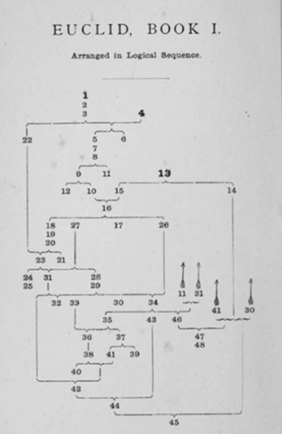
Figure 14.1 Frontispiece from Dodgson’s Euclid and His Modern Rivals
(Source: from C. Dodgson, Euclid and His Modern Rivals)
Personally, Dodgson was educated at home; early on, he showed a strength in mathematics, and he read prodigiously. His health was generally frail (throughout his life, he suffered from migraine headaches, as well as his stutter), and, although he tried sports, he was humiliated by his ineptitude. It seems he generally kept to himself, and he never married. But, certainly, he knew Christ’s Church well, as many scenes from Alice and his other books are caricatures of actual places on campus. It was the only college with which he had a formal affiliation. He studied there as a student, and, upon graduation, he was hired as an instructor of mathematics. He eventually rose to full professor and held that position for the remainder of his career. It is reported that he was an engaging instructor and popular with students and colleagues alike. He played chess and made up word puzzles that typically had some twist of logic. This penchant is seen throughout Alice’s Adventures in Wonderland. At least one book (though I suspect there are others) is devoted to presenting the puzzles of his literary works.
* * * * * *
A brief editorial note about sequencing events in our story is needed at this point. As readers recognize, I have generally introduced the people and events that contributed to quantification in rough chronological order. To continue that order, I would now introduce the early inventors and developers of psychological testing (IQ and achievement tests, mostly), including Alfred Binet, James Cattell, Théodore Simon, Lewis Terman, L. L. Thurstone, and David Wechsler. These individuals were important in bringing quantification to a broad populace through their work in this specialized field. However, their efforts spread over a relatively long period, stretching from the mid-nineteenth century to the mid-twentieth. Also, in this age, others were working in pure mathematics, statistics, and probability theory. It seems a bit disjointed to slavishly adhere to a strict chronological order, because that would mean jumping back and forth between those involved in psychological testing and the pure mathematicians (including probability theorists). Hence, I will postpone describing the originators of psychological testing, keeping them together in a later chapter (Chapter 16) devoted to that topic.
* * * * * *
Many readers are undoubtedly aware that a source of national pride for the Irish is its Guinness beer, brewed in Dublin on the same site since 1759 (with a 9,000-year lease at St. James’s Gate!). For many, drinking a pint (or so) is as much a statement of cultural identity as refreshment; and all know the long-running campaign “My Goodness, My Guinness” with the famous Guinness toucan. Posters and knickknacks of every imaginable variety promote the dark brew. Most know, too, that Guinness has a distinctive taste and when first poured (there is a protocol to even this act), the bubbles rise, leaving a thick foam head, rather than fall, as for most other beers.
More to our point, the Guinness empire has historically been a leader in introducing research in manufacturing processes and that is how the brewery plays into the story of quantification. In 1901, the first Guinness research laboratory was established to examine water quality, hops, and more. A promising young man named William Gosset worked in the laboratory. Gosset was asked by his superiors to address a specific problem: determining the optimal ratio of hard to soft resins in the hops used by the brewery to flavor the beer. Hops are the flower of the plant Humulus lupulus, containing both hard and soft resins. Their ratio is what determines a beer’s degree of bitterness, a necessary part of its flavor.
The brewery acquired hops from many sources, and Gosset realized that, in order to answer his primary question, he must first determine the consistency of the ratio across the many batches purchased. It is reported that, in one batch of eleven samples, there was an average 8.1 percent soft resins while, in another batch, from fourteen samples, the average was 8.4 percent soft resins. He certainly knew of the central limit theorem and that he could integrate the data into a cumulative frequency distribution. But, as we saw earlier, applying the theorem requires quite a few samples (considered to be thirty at minimum). He simply did not have enough samples to apply the theorem here. So, he formalized the problem as one of determining consistency across relatively few samples.
Gosset conceptualized the problem as one of determining by how much the values in his small sample differed from the normal distribution. Cleverly, he made his own version of the standard normal distribution (we saw the standard normal distribution in Chapter 9) by simulating many samples and specifying that it had a defined mean and standard deviation of 0 and 1, respectively; he called this the “z-distribution.” He took just two samples of his hops and compared them to his theoretically derived z-distribution; he then repeated this several times. To his surprise, he discovered that, in 80 percent of these comparisons, he was within 0.05 degrees of the true number (the term “degree” is a reference to the analytical geometry underpinning the statistical fitting of samples to a given distribution). In other words, most of the time, his comparison of these small samples to his standard normal distribution was quite close, although not exact. He repeated the whole thing with three samples and found that, now, 88 percent of the time he was within 0.05 degrees of the true number. When he used four samples, he was even closer. He repeated this two-sample comparison several times—enough to make a new distribution, which he called the “t-distribution.”
The t-distribution is more descriptive of small samples because of its slightly smushed shape: it looks like a bell curve that has been punched in on the sides so that the middle is higher and the tails are longer and flatter. By using a 0.05-degree criterion to test the difference between the t-distribution and the z-distribution, Gosset had invented a new approximation method that is useful when only a few samples can be had: the “t-test.”
To apply his t-test to varying research conditions, Gosset described three variations, including (1) a “one-sample t-test,” wherein the mean of a single group is gauged against a known mean, typically 0 from the z-distribution; (2) an “independent samples t-test” which compares the means for two groups; and (3) a “paired sample t-test” that compares means from the same group at different times, say, one week apart. These three types cover most common research scenarios.
Gosset wrote his findings in a report for the brewery, titling it “The Application of the ‘Law of Errors’ to the Work of the Brewery.” His Guinness superiors were thrilled with his work, for he had successfully addressed the problem originally posed to him, far beyond their original expectations. Gosset was a bright individual, and, although fairly new in his career as a researcher, he realized he was on to something. We know now, more than one hundred years on, he was indeed “on to something” because his t-test and t-distribution are standard fare in statistical analyses today. Their significance is captured by a historian of the period, who declared, “Very few achievements in statistics have been as momentous as Student’s [Gosset’s] discovery of the t-distribution” (Gorroochurn 2016a, 348).
Still, Gosset wanted to be sure of what he had invented. He needed to have someone verify his method. Even more generically, he also sought to devise a mathematical model for his method but was unsure of how exactly to do it. To this end, he requested a consultation with Karl Pearson of University College, London, who had a well-known mathematics laboratory. The consultation became an extended study: Gosset spent a year there. During this time, Pearson was taken by the young man’s interest in applying probability to address practical problems, and they developed a friendship that lasted throughout their lives, despite Pearson being thirty-three years the senior. We saw in Chapter 13 that, earlier, Pearson had had a parallel friendship with Galton, who was thirty-five years his senior. The friends were, in seniority, Galton, Pearson, and the younger Gosset.
Back in Dublin after his experience working with Pearson, Gosset wanted to publish his findings on his small-sample distribution approximation. He contacted his friend and mentor Pearson, who was editor of Biometrika, the premier statistical journal of the day (it remains so today). Pearson agreed to publish Gosset’s work, and it appeared in a now-famous article titled “The Probable Error of a Mean” (Student (William S. Gosset) 1908, 1). The paper was a touchstone in the development of statistical tests using a criterion. Ronald Fisher, another famous statistician whom we will meet momentarily, notes this in his praise of Gossett for giving impetus to all studies of distributions: “The study of the exact distributions of statistics commences in 1908 with ‘Student’s’ paper ‘The Probable Error of a Mean’” (Fisher 1925, 23). And, of course, distributional statistics is fundamental to research analysis today.
But, in a well-known quirk of circumstance, the article appeared not under Gosset’s name but under the pseudonym “Student.” Many readers (and students of statistics) will recognize Gosset’s work as “Student’s t-distribution,” and its interpretation as “Student’s t-test.” Figure 14.2 shows Page 1 of this famous article.
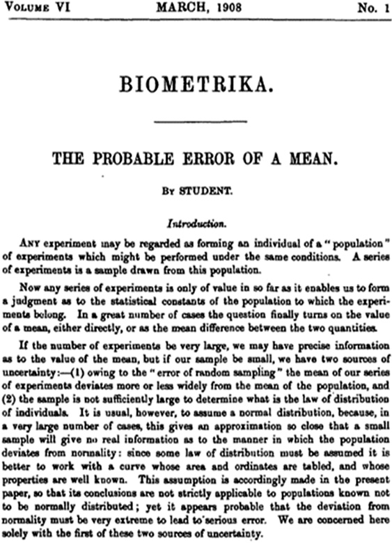
Figure 14.2 Portion of Page 1 from Gosset’s Biometrika paper published as “STUDENT”
(Source: Permission from Oxford University Press.)
Several reasons are speculated for why Gosset published under the pseudonym “Student.” None are fully corroborated, but all are fun to imagine. In one, the Guinness brewery wanted to hide from the competition that it was relying upon scientific approaches for decisions over using what was thought to be the wisdom of the senses garnered from generations of brewers. Another less folksy reason is that Karl Pearson made up the name and imposed it upon Gosset because, as founder and editor of the most prestigious academic journal of the day, he did not want to have his journal associated with a pub’s stock-in-trade.
And yet, what better way to discuss quantification than over a pint of Guinness!
* * * * * *
Gosset was a friendly, gregarious individual. As well as his friendship with Pearson, he had another professional acquaintance, this time with someone a bit nearer his own age, Ronald Fisher. Together, they worked on developing the t-distribution, eventually leading to its mathematical proof. Most of their contact was by letters written over an eight-year period in the 1920s; at least eighty of these letters survive for reading today (Box 1981).
The two men communicated by letter, rather than meeting in person, because they lived in Ireland and England, respectively, in a time when the politics of Irish independence dominated much of public discussion and governmental energy. Although not a long journey, travel between the countries was limited and not common beyond intragovernmental contacts. The Irish Nationalist Charles Parnell had, only a few years earlier, as an influential member of the British House of Commons, laid the groundwork for Irish independence. This was on the heels of the Potato Famine in the 1840s, when one million people starved to death, and nearly two million more fled to the United States or, if less well heeled, to Australia. All the while, the British sat idly by, ruling in Dublin just 100 kilometers (60 miles) to the west and doing almost nothing to help. The problems festered and finally led to the 1916 “Easter Rising” against British rule in Dublin, where vastly outgunned Irish protesters were shot in front of the Post Office (a noted civic building in the central part of the city). Soon, events turned revolutionary with the guerrilla-style Anglo-Irish War and its adherents in the Irish Republican Army (more commonly known by its acronym IRA), leading to the decades-long conflict known as the “Troubles.”
In 1921, a ceasefire was signed, and the country was divided into two parts, the Republic of Ireland and Northern Ireland, after the ineffectual Éamon de Valera’s inept negotiations with Great Britain for home rule. Unfortunately, this did not end the Troubles. The popular first chairman of the Provisional Government of the Irish Free State, Michael Collins, was assassinated just seven months into his term, and there was dissatisfaction about having the homeland divided. The Troubles continue to this day, in an ebb and flow, although now mostly isolated to Londonderry and Northern Ireland. Belfast remains a divided city.
Against this social and political backdrop, Gosset and Fisher maintained their friendship and collaborated on statistical developments.
Fisher was a British statistician of prodigious accomplishments. To many individuals, he is considered the “father of modern statistics.” This title is certainly true for the inferential statistics employed in so much of today’s research. A historian of early statistics opens a chapter on Fisher with this accolade: “‘Monumental’ and ‘revolutionary’ are words that come to mind when attempting to assess Fisher’s impact on mathematical statistics” (Gorroochurn 2016a, 371). Another statistician gives him this praise: “Even scientists need their heroes, and R. A. Fisher was certainly the hero of twentieth-century statistics. His ideas dominated and transformed our field to an extent a Caesar or an Alexander might have envied” (Efron 1998, 95). You can see, with Fisher, we are meeting someone important in quantification.
Further, readers may already know, too, that Fisher is the inventor of the famous “lady tasting tea” problem, which I will describe momentarily. (It sets the stage for modern hypothesis testing by statistical inference.) First, however, I give some background and context for Fisher’s accomplishments, although his achievements are so numerous I cannot describe them all. I will describe only some of Fisher’s work as it contributes to our story of quantification. Readers with a special interest in the history of statistics may wish to explore this titan’s work further, but I offer this bit of warning on reading Fisher’s original writing: his composition is endlessly awkward. I refer you to a good biography or summary of his work, such as that by Gorroochurn (2016a).
The relationship between Gosset and Fisher began when Fisher was still a student. He admired Gosset’s work and thought he had something to offer by suggesting a technical modification to better account for the “degrees of freedom” used with his t-distribution. “Degrees of freedom” is an important statistical concept that is best understood by working with it, even if only a little. It allows for estimating the alignment (called “model fit”) of observed data (i.e., the sample) with a hypothesized distribution, most often the normal distribution. The underlying geometry that is necessary to fully understand this concept need not concern us here; rather, what is important is that it is needed for the proper interpretation of research hypotheses because the number of subjects comprising a sample varies from one study to the next, and the concept of “degrees of freedom” allows for this variation.
For our purposes, Fisher’s modification with degrees of freedom strengthens Gosset’s t-tests. Further, Fisher’s work in this area also led him to his pivotal statistical invention of the F-distribution and the F ratio.
His work on Gosset’s distributions led Fisher to an acquaintance with Pearson, which unfortunately degenerated into a personal feud. I mention this because it may have inhibited Fisher from attaining even greater heights, and it shows that these notables were still human. While yet a student, Fisher sought to publish his work in Pearson’s journal Biometrika, the same journal where Gosset (as “Student”) published his important work, “The Probable Error of a Mean.” Pearson did publish young Fisher’s paper, which set Fisher’s reputation as a rising statistician. But, two years later, Pearson published an article criticizing Fisher’s work. Fisher was quite unhappy because he realized Pearson’s comments would be widely read among his circle, and he believed that the point of criticism was incorrect. It turned out that Fisher had got it right in the first place. He wrote a paper defending his original work and demanded that Pearson publish it. Pearson did so, but not as a separate piece; rather, he included it only as an appendix to another paper. This miffed Fisher greatly. Then, two others of Fisher’s papers were rejected by Pearson—much to Fisher’s growing anger.
Despite their personal tension, it seems that Pearson appreciated Fisher’s abilities: he offered him a very good job, that of Chief Statistician at the prestigious Galton Laboratory. Fisher, who apparently had not yet got over his bad feelings, refused. In fact, he vowed to never again publish in Biometrika, and, although, over the years, he developed several other important ideas, he kept true to his pledge, preferring to publish them in less impressive outlets.
But Fisher’s reputation was growing, and he was not without professional options. He secured a position as Chief Statistician at the Rothamsted Experimental Station, the first laboratory devoted exclusively to researching agriculture. (Rothamsted is a city located a bit north of London.) While there, he researched problems in soil types and plant fertility. This job fit with his interests in farming and in genetics.
All his life, Fisher suffered from extremely poor eyesight, which was debilitating, but when young, he turned it to academic advantage. His weak eyesight made him ineligible for military service. Britain needed conscripts during years surrounding several of its conflicts, including its colonial campaigns, the Irish Troubles, and tensions across Europe leading to WWI. Because he couldn’t serve, he had the opportunity to pursue academics—but, even more pointedly, because he could not easily read his mathematics texts, he was forced to visualize the subject, including memorizing formulas and entire tables. This unusual approach to studying gave him a perspective on the topic that few others had. It is reasonable to surmise, too, that it may have spurred on his imagination to conceive his innovative approaches to statistics and research designs. One never knows for certain from where creativity flows, but certainly Fisher had it.
While at Rothamsted, Fisher let his creative spirit fly, for he pursued all manner of studies on snails, poultry, and mice, and, seemingly with each one, he produced yet another modernization in statistical approaches and methodologies. He introduced the concept of randomized trials for experiments, and he designed experiments that had levels for each experimental factor, allowing for much more efficient testing. With such factorial experiments, several hypotheses could be tested simultaneously. If that were not enough, he devised his analysis of variance procedure to assess the viability of multiple hypotheses simultaneously. Each of these accomplishments is significant in itself. To think that all came from the creativity of one man—and in such quick succession—is testament to an astonishing level of productivity.
In 1922, he published a seminal paper titled “The Goodness of Fit of Regression Formulae and the Distribution of Regression Coefficients” (Fisher 1922b) in which he initially explored a distribution called the chi-square (χ2) distribution and regression coefficients. But this exploration led him to offer a wholly new perspective on analyzing data from samples: a ratio of variances. This ratio uses a variance statistic that is (inferentially, at least) accounted by the experimental condition compared to all of the variance in the experiment. As some readers may immediately recognize, this is the famous analysis of variance (ANOVA) ratio. The statistic later came to be called the “F ratio.” Before Fisher, no method had been devised to statistically account for differences between groups while simultaneously considering the amount of error. ANOVA’s full approach gives veracity to interpreting research findings. As most readers know, too, ANOVA is foundational to experimental methods used in today’s research. We look at this famous procedure momentarily.
Fisher continued innovating procedures and methods at an astounding rate. To cite one important article, “On the Mathematical Foundations of Theoretical Statistics” (Fisher 1922a), he lays out statistical vocabulary and concepts, including “efficiency,” “location,” “scaling,” “maximum likelihood,” and “parameter.” The quantity and significance of his many contributions is awesome.
A few years later, in 1925, he documented all these procedures in a remarkable book titled Statistical Methods for Research Workers (Fisher 1925). This book quickly became the standard text for research methods for many years. Fisher updated it in numerous editions throughout his life. In the introduction to a later edition, Fisher wrote about the success of this first tome, saying,
It is 25 years since Statistical Methods for Research Workers first appeared. Its importance to research workers in all branches of science is clear from the fact that it is now in its eleventh edition, and that translations have been made into French, German, Spanish, and Italian. (Fisher 1950, vi)
Today, more than ninety years later, its influence remains. Of course, the work has been overtaken by hundreds of complementary texts, yet virtually all of them include Fisher’s experimental designs and his analysis of variance. It is no wonder that some hold fast to their attribution of Fisher as the father of modern statistics.
Ten years on at Rothamsted Experimental Station, Fisher had performed hundreds of agriculture experiments. He was focused particularly on methodology, and he developed an entire structure for many experimental designs. In particular, he was interested in controlling error between groups, which he called “batch-to-batch variation,” as a refinement on Gossett’s work at Guinness with variation in resins in hops. He set out to develop procedures for experiments that would control for this variation. He was enormously successful in his quest.
While Fisher did not invent the concept of random numbers, he did introduce randomization to experimental design, making it an operational feature in experiments. This development was momentous at the time, and it survives today as an essential feature of valid experiments. In a genuinely random experiment, say, as in a “control group vs. experimental group” design, all of the subjects for a sample are selected at random from a population. Next, the sample’s subjects are randomly assigned to one of the two groups (treatment group or control group). And, finally, the treatment (called the “independent variable”) is then assigned at random to one group but not the other. This practice was Fisher’s devising, and it is the standard in use today.
When true randomization cannot be achieved but only an approximation of randomization is obtained (a common circumstance in human factors experiments), the experiment is labeled as following a “quasi-experimental” design.
Fisher had another important first in designing experiments: introducing the “null hypothesis” into research designs. This important feature is where a positive statement is not proved; instead, the unlikely occurrence of the opposite is rejected. This experimental design is called “hypothesis testing” or “inferential testing.” To give an example, suppose a careful scientist wants to prove that the sun will rise in the morning. The scientist proffers a hypothesis to this effect: “H1: The sun will rise in the a.m.” In Aristotelian logic, as well as in research contexts, a hypothesis like this cannot be proved directly. So, the researcher revises the original hypothesis into a second, opposite hypothesis, a null hypothesis: “H0: The sun will not rise in the a.m.” The experimenter then gathers data by observing that, for many days, each morning, indeed, the bright yellow-orange orb shows up over the eastern horizon. Using some statistical criterion to analyze the data, the researcher finds that the null hypothesis is unlikely. The conclusion is reached to reject the null hypothesis and infer that the original hypothesis (the sun will rise in the morning) should be accepted as true. Significantly, the research has not proven the hypothesis but has reached a conclusion by inference.
Fisher continued on his road of firsts by devising a statistical test to reject a null hypothesis. In it, he compared variances (this is the standard deviation squared) in a systematic manner. He analyzed the variances of an experiment, calling his procedure the “analysis of variance,” (referred to by the shorthand ANOVA). Likely, many readers have some familiarity with ANOVA, so my explanation here is brief. ANOVA is a ratio of two variances: the variance attributed to the experimental condition, and all of the variance in the experiment. The values for these variances are expressed in a “sum of squares,” which is itself divided by the experiment’s degrees of freedom to yield an average (the “mean square” for the sums) used in the ratio.
Mathematically, ANOVA can be written as an assumption wherein
![]()
This simple equation means that the sample observed value (for a random subject) equals the population mean plus some random amount of error. (Note that this is the ANOVA generalized form as an assumption and not the formula for the F ratio, which is its implementation with actual data.) The general formula is incredibly powerful. It is one of the most-used expressions all of research for comparing group differences. It is efficient, in that it can test several hypotheses simultaneously.
Because the ANOVA procedure is so common to research, in Figure 14.3 I present sample tables of the output procedure leading to the F ratio. Don’t worry about interpreting the tables, or even making sense of its columns—the purpose here is merely to illustrate tables that are universally known in experimental research.
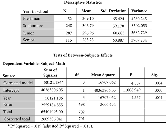
Figure 14.3 Illustrative output showing descriptive statistics and an ANOVA table
As you may have guessed, the “F” statistic is so named to honor Fisher. Well earned, Sir Ronald Fisher!
In modern statistics, the ANOVA has been extended into a more comprehensive tool in which differing contexts for the variable can also be considered. For example, suppose one is interested in investigating differences in teaching styles (e.g., supportive vs. authoritarian) on effectiveness in reading comprehension for late elementary school-age students (late primary level). Although the ANOVA can readily accommodate this type of between-group comparison, it does not capture much of the complexity of a real-world scenario. Suppose further, then, that one is also interested in considering contextual variables, such as the locale of the school (neighborhood socioeconomics: high vs. medium vs. low) or a student’s motivation (high vs. medium vs. low). These additional contrasts can be incorporated into Fisher’s analysis of variance in the advanced procedure “hierarchical linear modeling” (or HLM). This form of variance analyses is very popularly employed in sophisticated research problems.
Just to show you how HLM looks, the ANOVA comparison is now rewritten to focus on an individual’s outcome within the contexts mentioned (a linear regression model). The formula now is
![]()
You may recognize this as a special expansion of the binomial discussed earlier. Those early ideas do indeed carry forward! Don’t worry about working through it. (I suppose it is possible to work it by hand, but that would be ridiculously tedious—even silly—with today’s computers at hand.). As always in this book, my purpose with formulas is to just illustrate them so that you may see how they look, not to explain them didactically.
As mentioned earlier, Fisher organized his experiments according to their conditions for treatments, which he labeled “factors.” His factorial approach was instrumental to most of his research. There are many ways in which factors can be arranged in an experiment. One common arrangement is called a “Latin squares” design. Fisher did not invent the notion of Latin squares (that happened much earlier, probably with Euler), but he devised an entire typology of applying the concept to research designs. This is a clever arrangement of variables and factors that controls for unwanted variance (e.g., things that interfere with learning the true effects of an experiment). At Cambridge University, a stained-glass window illustrating a 7 × 7 Latin squares design honors Fisher.
Incidentally, those who enjoy working on Sudoku puzzles may be interested to learn that any solution to a Sudoku puzzle is a Latin square of Fisher’s devising!
* * * * * *
In storybook fashion, Fisher summarized his work, including introducing many research principles, like his Latin squares design, in a foundational book on research methods titled The Design of Experiments, which was first published in 1935. As with so much of Fisher’s work, this book is remarkable in many respects. For one, he presents a classic description of inferential testing, as we discussed above. He does this in Chapter 2 of the book, which he titled “The Principles of Experimentation, Illustrated by a Psycho-Physical Experiment.” This is the chapter that contains the famous story of the lady tasting tea.
It is most fun to see the story in Fisher’s own words. He describes the problem as follows.
A lady declares that by tasting a cup of tea made with milk, she can discriminate whether the milk or the tea infusion was first added to the cup. We will consider the problem of designing an experiment by means of which this assertion can be tested. For this purpose, let us first lay down a simple form of experiment with a view of studying its limitations and its characteristics, both those which appear to be essential to the experimental method, when well developed, and those which are not essential but auxiliary. (Fisher 1956, 11; also Fisher 1971, 1512)
And here is the experiment:
[It] consists in mixing eight cups of tea, four in one way and four in the other, and presenting them to the subject for judgment in a random order. The subject has been told in advance of that the test will consist, namely, that she will be asked to taste eight cups, that these shall be four of each kind. (Fisher 1956, 11; also Fisher 1971, 1512)
By this, there are ![]() distinct possible orderings of the cups of tea. This is computed from the fact that there are eight cups of tea: four had milk poured first, and four had tea poured first (see Figure 14.4).
distinct possible orderings of the cups of tea. This is computed from the fact that there are eight cups of tea: four had milk poured first, and four had tea poured first (see Figure 14.4).
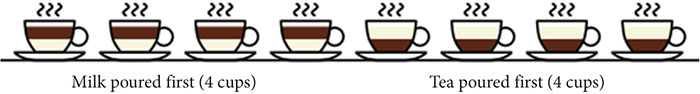
Figure 14.4 Illustration of Fisher’s research problem “The Lady Tasting Tea.”
(Source: http://commons.wikimedia.org/wiki/Category:Public_domain)
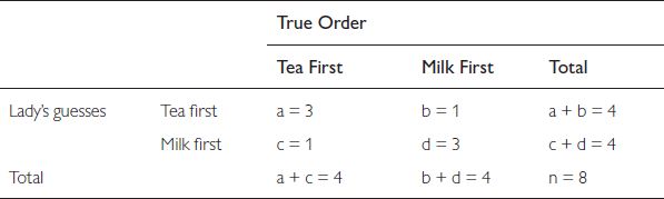
The possibilities can be presented in a contingency table as in Table 14.1. This table shows the number of choices made for the lady’s guesses by the true order (tea first vs. milk first).
Table 14.1 Order of experiments for Fisher’s “the lady tasting tea” problem
In looking at the problem, one realizes that there is more than one solution, each with its associated assumptions and varying implications—but it is outside of our purpose to explain them fully. For those interested, there are numerous websites and other publications devoted to “the lady tasting tea” problem. I presume most are useful and even fun to explore, but I offer a caution, because some explanations are inaccurate and others seem to be unnecessarily complex. It is a relatively simple problem in statistics—its importance lies in Fisher’s presenting it as a probability problem with a statistical solution, a first at the time.
In The Design of Experiments, Fisher presented a solution that is referred to as “Fisher’s exact method.” By his approach, the exact probability can be readily calculated for each of the seventy possible outcomes, although it would be a bit silly to figure them all (since most are near zero): three or four possibilities are common. The formula for Fisher’s exact probability is given as
Using values shown in the contingency table, the answer is ![]() , meaning that the lady has about a 23 percent chance of selecting the four cups correctly. However, there is a bit more to it than that. Fisher’s research hypothesis is a null hypothesis, which states the “empty” case: that is, “How likely is it that the lady cannot discriminate?” Or, rather, that she cannot correctly guess all eight cups, as one-in-seventy circumstances.
, meaning that the lady has about a 23 percent chance of selecting the four cups correctly. However, there is a bit more to it than that. Fisher’s research hypothesis is a null hypothesis, which states the “empty” case: that is, “How likely is it that the lady cannot discriminate?” Or, rather, that she cannot correctly guess all eight cups, as one-in-seventy circumstances.
Here, the values in our contingency table change slightly to a = 4, b = 1, c = 1, and d = 4. By Fisher’s exact probability, we see ![]() , or more than one in a thousand of all correct choices. By summing these possibilities, the probability is
, or more than one in a thousand of all correct choices. By summing these possibilities, the probability is![]() , or about a 24 percent likelihood of observing Fisher’s hypothesis.
, or about a 24 percent likelihood of observing Fisher’s hypothesis.
The “lady tasting tea” remains one of the most enduring stories for teaching probability and hypothesis testing.