CHAPTER 4
Finis origine pendet, the Roman poet Manlius wrote: “The end depends on the beginning.” With our story we know the end—people have a worldview characterized by quantification in thought and expression; a transformed Weltanschauung—before the beginning. As to its first phases, we have seen how observing—a conspicuously ordinary part of daily existence—broadened in scope along several steps, culminating in Mayer’s ingenious methodology to become observation—an empirical tool for scientific inquiry.
And important antecedents have come on the scene, such as Newton’s invention of modern calculus and his structural foundation to the scientific method, as well as Pascal’s intentional study of estimation, leading to his invention (jointly with Fermat) of probability theory for measuring uncertainty, something they devised when studying the problem of points. And, in broad society, education was advancing through the appearance of schools in most towns and villages, effecting a slow but solid rise in the rate of literacy.
But these antecedents are just that: a preceding circumstance. With only a few exceptions (those working in the sciences and the academic peers of the individuals we have discussed), the daily lives of ordinary people had not yet been impacted. Uncertainty, indeterminacy, and unpredictability were still the mindset. More broadly across society, people had not yet considered uncertainty as a calculable part of their lives and thoughts. But how could they? After all, the mathematics of reliable estimation and prediction had not yet been invented, and probability theory was only in its infancy, as an idea. Significantly, however, the seeds for the new perspective had now been sown, if not yet sprouted.
Most ordinary people of the day (the early eighteenth century) lived ordinary lives, despite momentous historical events surrounding them. Men worked as farmers or businessmen, as soldiers or clergy, as teachers, or perhaps in the trades. Nearly all women were occupied as wives, mothers to many children, and caregivers of the elderly, who were often their own parents. It was common for them to assist their husbands in some way or another. The life of rural peasants at this time is illustrated in a famous painting by Jean-François Millet, The Gleaners. It depicts three peasant women bending over to gather the grain left by reapers after the wheat harvest. This moving image is shown in Figure 4.1.
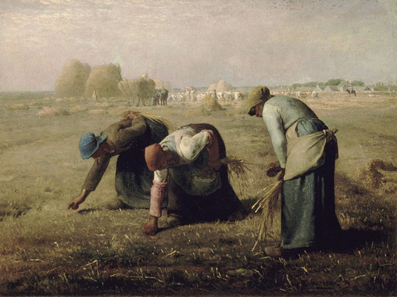
Figure 4.1 The Gleaners by Jean-François Millet
(Source: http://commons.wikimedia.org/wiki/Category:Public_domain)
All the while, the influences of quantification were in the air, suffusing people’s lives in subtle and yet unrealized ways.
In perhaps the most impactful event, both on an individual level and as progress toward quantification, more Europeans were learning to read. As mentioned, almost all towns and villages had at least elementary schools, and secondary schools were commonplace. Third-level education was well established by Oxford and Cambridge in England and Trinity College, Dublin. The Paris-Sorbonne University, an edifice of the Latin Quarter, was already centuries old. In the Nordic countries, Uppsala University in Sweden was famous for its scholarship, as was Universidad de Madrid. Across the sea, in the American colonies, Harvard College was by now more than half a century old, and two new promising colleges had been founded: William and Mary College in Williamsburg, Virginia, and Yale College in New Haven, Connecticut. As one can imagine from this, the emphasis on formal schooling was broad and deep, reflecting a new-found interest in learning, not only for its practical utility but also for the sake of bringing a richness to one’s existence. Learning for its own sake was gaining the appreciation of the populace at large.
Many newspapers had a widespread distribution, and local publications such as tabloids and political tracts were springing up regularly. The extensive availability of printed material contributed to spreading interest in reason and science, growing toward full expression of the Enlightenment. I mentioned earlier the enormous influence of the English translation of Newton’s Principia, most especially its Book I, on this period. While unlikely to have been read (due to its technical heft), Newton’s work was commonly known. During his lifetime, Newton was a renowned personality although he did not give public lectures beyond his teaching ones at Cambridge.
Virtually everyone held a deep belief in God or a higher being, and nearly all belonged to an organized religion, such as Protestantism, Catholicism, and Judaism. Only a tiny sliver of the population lived their lives apart from religion. Of a matter of course, the influence of the local pastor, priest, or rabbi on the daily life of ordinary people was weighty. Cultural and social life revolved around the local church, parish, or synagogue often literally.
During this time, too, the Italian family Stradivari (its most famous member was Antonio Stradivari) was making violins, violas, and cellos. These skilled woodworkers were known to have spent considerable time and care in selecting their woods. They used spruce for the top and maple for the back and neck, treating it with several types of minerals, including potassium borate, and applying a finish composed of still-disputed ingredients. Their craftsmanship was of such skill that it still amazes everyone who examines it. And, of course, listening to a talented musician play on a Stradivarius is an awesome experience.
Global commerce, especially by sea, was commonplace after Captain (William) Kidd, the last of the Barbary pirates, was hanged in London in 1701. (Many folks hoped that his last words would be to reveal the location of a much-rumored buried treasure, but alas, not so.) His capture and trial attracted massive public interest and was symbolic of the end of a freewheeling lifestyle, whether lived out on the sea or on land. Not only were the seas now relatively safe, but, with Kidd’s unsuccessful attempt to bribe his way to freedom, public order was seen as firmly in place.
But all was not peaceful. The climate of the day—social, cultural, political, and intellectual—was fraught with disquieting influences. Forces leading to the French Revolution were building, and the colonists in America were fighting for secession from England. In the Queen Victoria period, the newly formed Great Britain (England had just incorporated Scotland and Wales into its sovereignty, following its domination over Ireland) declared war on France to stop the union of France and Spain. In Russia, the twenty-four-year-old Peter (later Peter the Great, of the House of Romanov) became the sole tsar (later emperor) of Russia and almost immediately let loose his expansionist dreams, an aggression that lasted for decades and set the course for nearly two centuries of poverty for his people and societal unrest throughout northern Eurasia. While he did bring some stability to a chaotic government, he focused his reforms on building Russia into a military power, rejecting the developments of the Renaissance and the Reformation, and he kept Russia isolated from the rest of the world. These forces inhibited intellectual development in that part of the world.
* * * * * *
Although yet early in our story, we already realize that probability theory leads us through the unfolding of quantification because, primarily, this is the methodology for assessing uncertainty. As the methods of probability theory are invented and grow in sophistication and utility, we will see that adopting quantification as a worldview in ordinary folks is quick on its heels. With this as context, then, it is to Pascal and Fermat’s newly invented probability theory itself that we now turn.
As emphasized in Chapter 1, I describe each mathematical achievement only to advance our story and not as didactic explanation. Readers familiar with probability theory will realize that I leave out much information about each procedure that is given in textbook explanations. Remember, our story is about people, not methods.
* * * * * *
Like all things quantitative, probability theory relies upon some basic rules for numbers. Through the course of time, some of these rules have been codified into mathematical theorems, or statements accepted as fact. It’s important to know that theorems are mathematically verified, typically by an algebra or calculus proof. Virtually all branches of mathematics rely upon theorems, and mathematicians, researchers, and other practitioners generally assume the theorems in their work and often cite them when interpreting their evidence for a particular finding or conclusion.
Three simple theorems—the binomial theorem, the law of large numbers, and the central limit theorem—are fundamental to how numbers operate in a probability circumstance. Although each theorem carries unique information, they are closely related, like the separate movements of a complete symphony. They coalesce to form a sophisticated mathematical underpinning for the whole theory. The binomial theorem builds to a special case in the law of large numbers, which is itself closely related to the central limit theorem.
These profound theorems are undoubtedly the most useful—and used—theorems in probability theory and perhaps in all of mathematics. They are truly that foundational. Any strong mathematician (and certainly most persons working in statistics or probability theory) will recognize them immediately. As we examine the theorems, don’t be surprised if you have a sudden epiphany that they present common-sense ideas. In fact, they do! Their beauty lies in their simplicity and clarity. Here we see that the best ideas are also the simplest. Further, even though we will not look at the proofs of the theorems, know that these too are relatively straightforward. However, this is not to imply that we can gloss over them or be glib in our understanding. We should attend to their meaning with care. This is an instance where meticulousness in understanding matters.
I will explain each theorem in nontechnical language, emphasizing its relevance to quantification. As we go along, I also show the mathematical formula for each theorem—but just so you can see how they look. Certainly, we will not derive them, prove them, or even explain their math. A mere glance at them will serve our purpose.
We start with the binomial theorem, because it is the oldest, and then move on to the others.
Newton is credited with developing the modern version of the binomial theorem, although it has roots dating clear back to Euclid and probably before him. There is record of its ideas existing in early Europe, in China, and in India. Omar Khayyam, the eleventh-century Persian mathematician and poet–philosopher, is known to have worked with binomial expansions. But these early versions appear to be much less developed than Newton’s formulation. Hence, we acknowledge that the idea of the binomial, and binomial expansions, has been around for quite some time, but our work begins with Newton.
Despite its long history, the binomial theorem is not stodgy old math; indeed, it is pertinent today, even dramatically so. For example (as you may be surprised to learn), the binary logic of computer code that has found application in the opening and closing of electronic pathways on circuit boards and microchips is firmly grounded in the binomial theorem. Without it, there would be no branching for computer combinatorics, the arrangement of numbers as groups of logic that move around on a circuit board.
As another example of its relevance, electronic transfers of money—the core of our monetary system, happening millions of time each day such as with credit card transactions, across the globe—use binomial expansions in their algorithms. The binomial theorem is, literally, quantification in our daily lives! We return to this amazing realization several times throughout this book.
Further, the binomial theorem appears in some other, unexpected places, like literature. One fun example is when we see it in the stories of Sir Arthur Conan Doyle, who created Detective Sherlock Holmes, of the second most famous address in London: 221B Baker Street. Fans of the amazingly observant detective know that his archenemy is Professor James Moriarty, the “Napoleon of crime.” In the story The Final Problem, the young professor carries with him a book he wrote that is a teasing curiosity throughout the story because there are frequent hints that it may contain clues to the murder mystery. Professor Moriarty’s book is a treatise on the binomial theorem! The “consulting detective” (as Sherlock is called in the stories) mentions it when describing his nemesis:
He is a man of good birth and excellent education, endowed by nature with a phenomenal mathematical faculty. At the age of twenty-one, he wrote a treatise upon the binomial theorem, which has had a European vogue. On the strength of it he won the mathematical chair at one of our smaller universities, and had, to all appearances, a most brilliant career before him. (Doyle, Morley, and Mottram 1981)
Huh! Who would have imagined that there is a connection between the binomial theorem and Sherlock Holmes? We will see many more such gems as we go along in our story.
Now, on to describing what the binomial theorem is and how it works. In algebra, a binomial is just two terms that are either added or subtracted together. The simplest binomial expression is a + b. Obviously, bi means two, for its two terms. They can be slightly different; for example, 3x + 4 is another binomial, as is 2a(a + b)2, and so forth.
The binomial theorem is a clever formula specifying how numbers can be combined in many useful ways, including the powers of sums, in permutations and in other arrangements. For explanation, in mathematics, a “combination” is when numbers are considered together and their order does not matter; a “permutation” is when the order does matter. Thus, a permutation is an ordered combination. These arrangements allow for numeric expansion, meaning an equation can be manipulated by, say, multiplying it by itself.
Now, I will show the binomial theorem as a formula, just so that you may see what it looks like. As promised, we will not work with it at all. If this is uncomfortable territory, just skip over the formula—doing so will not interrupt the story—and pick up at the paragraph below it.
The important aspect to notice in the binomial theorem is the left side of the equation: particularly, that it is just two terms added together (a binomial). The exponent n means that the two terms can be expanded (i.e., squared, cubed, etc.). This is the general form for binomial expansions (different texts vary the notation):
Imagine solving this equation manually, a couple of hundred years before calculators were available. For the simplest binomial expansion (its square), the solution is not too difficult, but with more expansions it is exceedingly hard. The computations grow in length and complexity with each level of expansion. This is tough sledding.
Here are just three multiplying expansions of the binomial a + b. Note particularly that each expansion is that much longer than the previous one, and a lot more tedious to compute. The third expansion is longer yet:
![]()
![]()
and
![]()
Imagine the next few expansions of the binomial: that is, bring them to the fifth power or the ninth power. Each time it is expanded, the results grow longer and longer, ever increasing in complexity and cumbersomeness. The calculations (remember, at the time, done by hand) are certainly possible but exceedingly tedious, probably taking hours, and they would be pages long. And that is presuming no mistakes along the way.
Fortunately, Pascal invented a graphical arrangement of numbers that makes it a lot simpler to determine many expansions of the binomial. This famous graphical portrayal is Pascal’s triangle. Like the binomial itself, Pascal’s number arrangement has a prior (but unclear) history, but Pascal is credited with this form. Here, a picture really is worth a thousand words. As seen in Figure 4.2, Pascal’s triangle is a triangular array of numbers starting with 1 at the apex and with each subsequent row starting and ending with 1. Each of the remaining numbers is the sum of the nearest two numbers in the row above.
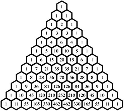
Figure 4.2 Pascal’s triangle
Working with Pascal’s triangle to calculate binomial expansions is rather like a logic puzzle or a game, wherein the numbers needed to solve an expansion are given as coefficients and exponents. Coefficients are numbers that go ahead of the variable and is a multiplicative factor. For instance, in 2a + b, the 2 is a coefficient stipulating that the a is to be multiplied by 2. Of course, an exponent is the number of expansions.
In the triangle, after the apex 1, turn your attention to its first row: 1 and 1. These values are the coefficients for the binomial’s first level a + b; that is, this could be written (rather unconventionally, but to make the point) either as 1a + 1b or as (a + b)1, meaning 1 times a and 1 times b. Of course, it is more conveniently just a + b.
Next, consider the binomial expansion when squared: (a + b)2. To solve this expansion, look to the second row in the triangle: 1, 2, 1. These are the coefficients for a2 + 2ab + b2. (For the exponents, count up the boxes above each number.) The process iterates for each level of expansion.
In advantage over Newton’s formula, Pascal’s triangle provides a much simpler way to solve these combinations, regardless of the number of expansions (at least up to a point). Realize, however, that Pascal’s triangle is not a shortcut for all expansions and permutations of the binomial; it only works for some of them. Complications arise with negative exponents, for example. For these advanced expansions, Newton’s binomial formula is still needed. Of course, today any mathematical calculation for binomial expansion (e.g., when done with calculators and computer programs) is accomplished with Newton’s binomial theorem, not Pascal’s triangle. But is does not matter, as the result is the same. Imaginably, most of the time, Pascal’s triangle was a lifesaver to persons in our pre-calculator story.
* * * * * *
The next two theorems, the law of large numbers, and the central limit theorem, concern populations and samples. Both theorems address the issue of how samples can be used to represent a population. And, commonly, but not exclusively, they are employed in research contexts. In probability, a “population” refers to the total set of observations that can be made. For example, if the interest is, say, a population of all persons with diabetes, then everyone with the disease, regardless of its type and stage, is included. Or a population can be something organic, like a plant or a microorganism, or something inorganic, like a mineral. Nearly anything can be a population here. However, it is essential in research that an exact description be determined. An imprecise description of a given population is a common reason for misinterpreting findings.
A “sample” is just those members of the population from whom information is collected, whether by observation, a questionnaire, a test, or some other record. Virtually always, the primary concern with samples is to ensure that they represent the population accurately and completely, something easier said than done. Simple random sampling is one common strategy for selecting participants, but there are many other selection methodologies, too. Later on, especially when we meet Sir Ronald Fisher, we will explore a few of them—some are rather clever.
With these terms now known, we can discuss the next two theorems.
The first is the law of large numbers. By the law, the more that is known about an event by repeating its occurrence, the more likely one can estimate the “true” outcome. The true outcome is the theoretical finding that would be obtained if everyone in the prescribed population was included in the probability consideration, and there were no errors from any source. Learning the true outcome is the goal of every such project. In reality, however, it is exceedingly rare when all persons in a given population are included. Hence, samples are taken.
Here is where the two theorems come into play. The law of large numbers tells us that the average value of many samples—in fact, ever more and more samples—will converge to be the same as the true outcome: there will be no difference between the two. That is to say, the more samples we have, the closer will be the average value of those sample statistics to the true outcome.
This idea is most easily seen through an example. Imagine a research project in which a medical researcher tracks adult women who have been diagnosed with osteoporosis. A bone-density T-score of −2.5 or below is a diagnosis of osteoporosis (−1.0 or above is normal bone density). For the theorem, this threshold value of −2.5 is the true score, in this case. The first group of subjects is comprised of twenty-five women whose average T-score is determined to be −2.8. Thus, their value is not representative of the threshold “true” osteoporosis diagnostic value. With a second group of twenty-five women, the average T-score is far above the threshold—say it is −2.0. Taken together, the two groups have a combined average T-score of −2.4—still, not exactly the true score. The third through sixth groups have T-score averages of −2.6, −2.4, −3, −2.1, respectively. Each time, a cumulative average score is computed. The point for the law of large numbers is that, over many trials, the cumulative average value of the separate sample averages will converge to the true value, despite that fact that the score of any one of the trials may not be near the true value.
This data is shown in Figure 4.3. Note that some of the values in the figure are higher than the true outcome, while others are below it, but none is exactly the true −2.5. In this example, even with only six trials, they average to −2.483. With more trials, the average would grow ever closer to the true value of −2.5.
Figure 4.3 Varying group averages whose mean converges to the true score by law of large numbers
Now, we can understand the law clearly: the law of large numbers states that the more trials we have, the closer the two values: sample observed and population expected (true). This implies—importantly and usefully—the fact that one begins an experiment with little known about what to expect, but, by taking averages of subsequent trials, the true outcome can be predicted with a high degree of certainty.
The law of large numbers was invented by Jacob Bernoulli in 1713. We will learn more about him momentarily. But first we look at his own example of the law, which has become quite famous.
Bernoulli filled a jar with 5,000 pebbles: 3,000 red ones and 2,000 black ones, for a 3:2 proportion. He hypothesized that the probability of drawing samples of red- and black-colored pebbles from the jar would grow increasingly closer to the exact proportion of each color of pebble in the jar originally (3:2) as ever more samples were drawn. To prove his hypothesis, he sampled the pebbles from the jar by taking them out one at a time and placing them on the table. Each time, he noted whether the pebble was red or black. He saw that any given draw would not be predictable, but as he drew out more and more pebbles, the proportion of red to black pebbles on the table grew closer to the overall 3:2 ratio, as he predicted.
Bernoulli believed the expected (or true) value would emerge gradually in a back-and-forth convergence process wherein each successive trial would have less and less error, although, throughout, some of the errors would be above the true mean, and others below it. He labeled the entire phenomenon “reversion to the mean.”
This convergence to an average (and true) value was explored more fully by Sir Francis Galton about 150 years later while he was researching intelligence in children. He established its place in social science and renamed it “regression to the mean.” (We meet Galton—an interesting person himself—later on, in Chapter 12.)
As an idea, the law of large numbers is deceptively simple, leaving one to imagine that it is modest in its significance and perhaps even trivial. But there is a lot more to it than that misconception. It presents a concept that is pertinent to the very base of mathematics—namely, the why of an outcome. Solving a problem in probability or statistics (indeed, throughout all of mathematics) is one thing, but explaining why that outcome can be expected is quite another. Knowing why it is happening gives meaning to the problem. Bernoulli’s law of large numbers provides this why—that is what makes it so important and consequential. In fact, it is sometimes called the “golden theorem.”
The law’s mathematical expression is given in a formula. As with nearly all formulas in this book, it is displayed here so that you may see what it looks like, not that I will explain it, and, certainly, we will not work with it all. As before, do not worry about the formula itself—if you like, you can skip over it without any loss in our story. I show it in two forms: as it is most often seen in textbooks and then as a probability convergence (it has two theoretical versions, called “strong” and “weak”):
Simple strong form:![]() for
for ![]()
As probability:![]()
It took Bernoulli nearly 200 pages to explain this idea and work through a very laborious proof. To our modern minds, this seems cumbersome, but remember Bernoulli was the first to do it, and he had many issues of mathematics and logic to work through. Over the years, our proofs have become much more efficient (with other, supporting theorems available) and modern texts explain the law in about four or five pages. Actually, the probability convergence can be proven with just a few steps, requiring only about a page to illustrate.
The law of large numbers highlights yet another important notion in numeracy: that of accuracy of measurement. This belief follows from early astronomers’ debate of whether to use the single “best” observation or the mean of several observations, and then settling eventually on Mayer’s method for combining observations. But because of Bernoulli’s work on his law of large numbers, this debate was advanced with his developing the first principles of the calculus of variation, now referred to as “measurement error.” And as we will see later on in this chapter, this is also the focus for Laplace’s study.
As probability theory evolved in depth and sophistication, measurement error turned out to be an elemental concern. Measurement error accommodates variation among the samples. To Bernoulli, the whole notion behind his calculus of variation, indeed, his whole law, was just one of applying common sense, something anyone (even without the benefit of training in mathematics, he thought) could do. He churlishly said,
For even the most stupid of men, by some instinct of nature, by himself and without any instruction (which is a remarkable thing), is convinced that the more observations have been made, the less danger there is of wandering from one’s goal. (Quoted in Stigler 1986, 65)
Point taken, Professor Bernoulli. Sounds like empathy was not his strong suit.
As we saw, Bernoulli initially used games of chance for his illustrations, but he soon added examples from other fields. His used his law to predict the true ratio of male to female births in a population of live births, for example. Expanding probability work beyond just gambling was novel and proved to be important in itself, helping to establish probability as a discipline with broad application.
* * * * * *
Now, a bit about Jacob Bernoulli himself. He was also called James or Jacques. I note his first name particularly because he was a member of a large family that included several renowned mathematicians, perhaps as many as twelve. The most notable of the Bernoullis are Jacob, Johann, Daniel, and Nicolaus. We explore Jacob’s contribution to quantification first; later, we will meet others in this famous family. Unfortunately, the family was often preoccupied with their domestic rivalry, a circumstance that historians believe lessened their potential for even greater contributions to mathematics.
Surprisingly, when Jacob invented the law of large numbers, he had not intended to work on probability per se. He was more interested in exploring Leibniz’s theories on both integral and differential calculus. As mentioned earlier, Leibniz came to his own inventions of calculus independent of Newton, although his was somewhat later; and, yet further on, he advanced the original work of Newton by supplying proofs in a series of important but very difficult to understand theories. Jacob and his younger brother Johann were apparently undaunted by the mathematical complexity of these obscure proofs, and they began to study them in detail. They provided many of the missing particulars to Leibniz’s work, making calculus a much more complete procedure.
Bernoulli intended to publish his law of large numbers in a treatise he titled Ars Conjectandi (The Art of Conjecturing), but, unfortunately, he died before finishing it, relatively young at fifty years of age (Bernoulli 1968). It was published posthumously in 1713 by his nephew Nicolaus I. Bernoulli.
As is obvious from the title, Ars Conjectandi was written in Latin, the language of most mathematical treatises of the day, but, interestingly, the early translation into English and German was not The Art of Conjecturing, as one would guess it to be, but Probability Theory. This name stuck, and thus started the name “probability theory” for this new estimation discipline. Incidentally, a first edition of this work was recently put up for a rare books sale at a beginning auction price of $40,000.
Bernoulli famously extended his work with the law of large numbers to human behavior, which he was convinced was just as important in his law as anything else. He reasoned that not all things are equal in value to everybody. Bernoulli suggested there is a moral aspect to the choices people make. For example, he conjectured that if a poor man has but one dollar, it is very important to him because it may be just enough to buy his next meal or maybe a place to sleep that night (using money’s value in Bernoulli’s time). But if a rich man has a dollar, it is much less important since the loss of a single dollar would not change anything for that man. By this reasoning, Bernoulli added another kind of expectation about how people make choices, which he called a “moral expectation.” In Bernoulli’s words:
The determination of the value of an item must not be based on its price, but rather on the utility it yields. The price of the item is dependent only on the thing itself and is equal for everyone; the utility, however, is dependent on the particular circumstances of the person making the estimate. Thus there is no doubt that a gain of one thousand ducats is more significant to a pauper than to a rich man though both gain the same amount. (Bernoulli 1954, 26)
This moral expectation is instrumental to the story of quantitative thinking because it bridges—however early in development our overall story is at this stage—the mathematics of probability in the law of large numbers with everyday human behavior. Bernoulli used observation to formulate his law and then extended it to human behavior rather than leaving it solely in the realm of mathematicians.
The bridge between the law of large numbers and human behavior in his moral expectation was explored yet further by Bernoulli. He contrived some examples of the two effects when applied to gambling. He believed that the observed value (from the samples) will grow toward infinity (the expected value) for a rich man much sooner than for a poor man because the rich man can afford to make more bets (in effect, take more samples) and hence make more informed choices as he goes along.
As Bernoulli showed in his law, with the rich man’s opportunity to make more choices, his observed values will grow closer to the expected value (a sure thing in gambling) than for the man with just one dollar and fewer samples. Thus (in his theory), the poor man will be risk adverse, since the one dollar means everything to him. Again, using Bernoulli’s words:
Now it is highly probable that any increase in wealth, no matter how insignificant, will always result in an increase in utility which is inversely proportionate to the quantity of goods already possessed. (Bernoulli 1954, 25)
This is an “inverse probability,” something that we see more of later on in the story.
This dilemma between number of samples—more for the rich man but fewer for the poor man—changes the accumulated knowledge, because, as we saw earlier, having more samples means the observed values are closer to the expected value and, hence, closer to a winning bet in gambling. The question becomes: “How many samples will be taken by a random individual whose wealth is unknown?” Bernoulli reasoned that the criterion for making such a decision is naïvely done if it only considers the population expected value and not also the moral expectation. This famous problem is called the “St. Petersburg paradox.”
The St. Petersburg paradox was introduced by Jacob but formally presented as a probability problem by his nephew Nicolaus Bernoulli and still later was mathematically resolved by another of Jacob’s nephews, Daniel Bernoulli (brother to Nicolaus) in the Commentaries of the Imperial Academy of Science of Saint Petersburg, naming the host city for the conference where Nicolaus made his celebrated presentation (Bernoulli Society 1990).
Today, economists study the St. Petersburg paradox as integral to most economic theories in a classic risk-versus-reward scenario given in Daniel Bernoulli’s publication. For us, it makes quantitative thinking more real, because the dilemma is not an obscure problem of integral calculus but one that includes everyday human behavior. People think quantitatively when gambling, of course, but, with the introduction of the St. Petersburg paradox, it is evermore formalized as a quantifiable entity and brought closer to ordinary folks. Risk and reward are considerations in many decisions, but when the problem can be stated mathematically to calculate likely outcomes, the dilemma is reduced considerably. Quantitative thinking for everyone was coming into being, even in those early years.
Connected to the law of large numbers are two follow-on notions: the “law of averages” and the “gambler’s fallacy.” Neither is a mathematical theorem with a formal logic and proof. They are lay terms used to express a belief.
The law of averages, also by Jacob Bernoulli, states that because there is a chance for all the possibilities for an event, it is inevitable that, over some very large number of trials, any one of the possibilities will happen. For instance, there are six sides to a die, and if it is rolled over and over again, in the course of time, a particular side will inevitably show as up. Suppose a gambler wants the side with two dots to show as up. If the die is rolled enough times, because two is a possibility, the die will eventually show the two dots. It is not one in every six rolls: it may be on the first roll or it may be on the millionth roll, because any particular roll is random and all roles are independent. But, be patient, dear gambler—the two dots will inevitably show! Or maybe not. The die has no memory or reasoning capacity to give impetus for the two dots to land up.
In fact, this is why the law of averages is a fallacy and has no satisfactory mathematical proof. For the person who desires a given lottery number to show, say their birthdate … well, you get the idea.
The other closely related notion is the gambler’s fallacy (also called the Monte Carlo fallacy), although it was not developed by Bernoulli (which matters little, in this case). It is often associated, and mistakenly confused, with the law of large numbers. The gambler’s fallacy is the belief in hope itself: that is, because something has not come up among many trials, it is bound to happen soon—like on the next roll of the dice or the next spin of the roulette wheel. It is the reason people stay at a gaming table. (If you are looking for a reason to leave the table, reread the preceding paragraph on the law of averages.) The gambler’s fallacy keeps Las Vegas casino owners happy and, sadly, is the ruin of many relationships.
* * * * * *
Now, we come to the last theorem discussed in this chapter, the central limit theorem. It is the most profound of all the theorems we have seen; indeed, in all of probability theory and maybe even in all of mathematics. It is that appreciated, well known, and used. The central limit theorem is very neat and simple; yet, it applies to nearly all probability and experimental situations.
This theorem is closely related to the law of large numbers (the two are often confused) but it is distinct. The law of large numbers tells us that the average of samples will converge to the true (or expected) value, while here—the central limit theorem—we are concerned with the shape of the distribution of the samples. It addresses the question, “Can I make a bell-shaped curve by plotting the values garnered from the sample trials?”
In 1810, Laplace was examining the law of large numbers, and he reasoned that the mean value from a series of experimental trials is not a precise statistic but actually falls within certain limits. He interpreted the true value as itself a probability, even in the infinite case (e.g., the theoretical zillion times). He saw it as a problem of studying errors, positive and negative, “about” (meaning “above” and “below”) the mean. He proved that their mean result converges to a “limit” in a precise way. This sounds technical but we can see it more simply, as follows.
The central limit theorem states that, with certain conditions (such as adequate sample size), when many independent trials are taken, their means will approach a bell-shaped curve, regardless of the fact that any single trial may itself not be this symmetrical shape. It is useful to be reminded that the central limit theorem is concerned with the shape of the distribution composed of many samples.
A simple example will make it easy to see the theorem. Suppose a researcher is interested in exploring the variable of annual household income. In this study, the researcher simply asks people their annual household income, as self-reported. He visits several locales in the area and approaches people at random. Each time, he gathers data from the same number of people, say, five individuals. A visit to an area is a trial, and all values for that trial are the “sample.” For convenience, I will display the findings for each trial in a table (Table 4.1). Collectively, these numbers are called “sample statistics.”
Table 4.1 Annual household income for three locations
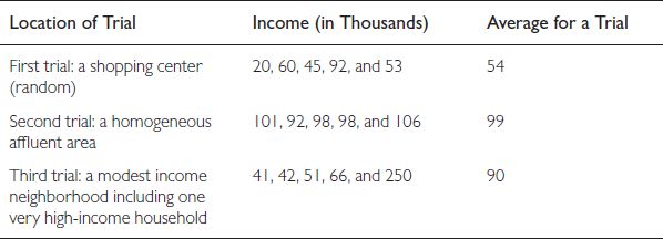
I use only three trials to keep things simple, but, in probability theory, about thirty trials would be a minimum to meet assumptions of the theorem (up to infinity would be better). Now, look closely in the table at the individual values for each trial, shown in the middle column, labeled “Income (in Thousands).” For the first trial, they appear to be random; in the second trial, they are relatively uniform; and, in the third trial, they are skewed by the one very high value.
The central limit theorem stipulates that—and this is the important point—regardless of how divergent any individual sample is from a normal distribution, the averages themselves (in the rightmost column) will converge to a normal distribution. Hence, plotting the values 54, 99, 90, and so on will create a bell-shaped curve, or, more technically, a normal probability distribution (called a “density function” when calculated by integration—I explain this notion more fully in Chapter 9 during the discussion of Gauss’s accomplishments).
As can be seen, the central limit theorem is concerned with the shape of the distribution, which is enormously important in nearly all research. Perhaps its greatest implication is that when its conditions are satisfied, research gathered from samples (individual trials) is generalizable to an entire population. After all, obtaining conclusions about populations is what makes research valuable.
In parallel with showing you the formulas for the two preceding theorems (the binomial theorem and the law of large numbers), I will show you the formula for the central limit theorem. It is given here, in two ways. First, I show it as integral calculus (this is what Laplace derived and then proved). Then, I give its essence in two parallel, much simpler forms. In textbooks, the former equation is shown in advanced texts, while the latter expressions are used in more elementary ones.
Remember, these formula displays are just so you can see what they look like and to give you a feel for what is involved. Obviously, providing an explanation would be lengthy and far off-track. You can just skip over them if you like, and pick up the text immediately below the formulas. You will not miss anything in our storyline.
As integral calculus, the central limit theorem looks like this:
(For the mathematically advanced reader, Laplace initially assumed that the error distribution could be ±1 with equal probability for each. And he started with the binomial (1 + 1)2n.)
More simply—and as commonly seen in most beginning statistics texts—the idea of the central limit theorem is given in these two expressions:
![]() (the sample mean equals the population mean), and
(the sample mean equals the population mean), and
![]() (the sample standard deviation equals the population standard deviation).
(the sample standard deviation equals the population standard deviation).
(Note: If you skipped the formulas, here is where to pick up again.)
* * * * * *
Quantification occurs in nature, too, a point not missed by Jacob Bernoulli. He made many calculations around natural objects, being among the first to recognize that natural structures can be modeled mathematically. Consider the Nautilus shell. A picture of one is shown in Figure 4.4. Doubtless, we all appreciate its near-perfect shape, its symmetry, and its sheer beauty. We are drawn to it almost supernaturally. Just seeing a picture of a Nautilus shell conjures emotions for something soothing and relaxing: it is comforting, peaceful, gentle, and even magical. But what draws us in is more than just its surface beauty. When we look at the Nautilus shell, we can see that its form is regular and predictable. It is not random or uncertain. Its spirals curl systematically.
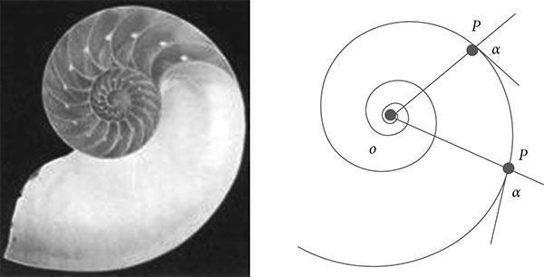
Figure 4.4 A Nautilus shell and Bernoulli’s logarithmic spiral
(Source: http://commons.wikimedia.org/wiki/Category:Public_domain)
Bernoulli called this shape the Spira mirabilis (for centuries called the “wonder spiral” and often now called the “golden spiral”) and is given credit for specifying the shell’s spiral shape as a mathematical arrangement of ratios, although he was not the first to do so. A few years earlier, René Descartes had also worked out a mathematical specification.
Bernoulli was transfixed by the special spiral. He realized that the spiral shape of the shell can be construed as a series of ratios which combine to form an arc that constantly reduces along the spiral’s length. Bernoulli saw it as a problem of integration (i.e., integral calculus). When so construed, one can figure dimensions for varying ratios at given points along the spiral’s length. The amplitudes of the angles defined by the lines and the corresponding tangents to the shape are of a constant value specifying its size. Because of these characteristics, it is an equiangular spiral.
These diminishing ratios are best expressed in logarithmic units. (Logs are a much easier metric to use for calculating the special relationship among ratios.) Bernoulli was so taken by the logarithmic spiral that he instructed his heirs to carve it into his tombstone. Not surprisingly, the measurements for the spiral shape occur in many other places, both in nature and in man-made forms. The starry arms of spiral galaxies often have the shape of the logarithmic spiral. And low-pressure systems of hurricanes, when viewed from space, are generally the same shape.
The ratios also relate to several other famous mathematical ratios and numbers, including Fibonacci numbers, the “golden ratio,” and the “golden rectangle.” In addition, it follows the form of patterns in our lives that are called “sacred geometry” patterns. We return to these special forms later on, since they do play an important role in the story of quantification as a worldview. Sufficient for now is to appreciate that, with Bernoulli’s work, we know the universe can be described in numbers.
A famous example of formally employing the equiangular spiral shape in one’s work is given us by Sir Christopher Wren, a seventeenth-century architect who was renowned for designing simple but elegant churches. He incorporated the spiral design into some of his structures, a few of which have survived to today. One small especially beautiful church he designed was located in a section of London that was to be rebuilt after Hitler’s WWII London bombings. It was decided that, instead of the church being demolished, it would carefully be disassembled, stone by stone (with each one given an identifying number) and then transported to the small American Midwestern town of Fulton, Missouri, where it was rebuilt to its original glory.
Of course, Wren did not use the term “quantification,” but, through this beautiful church’s structure, we see this idea moving into the realms of experience for ordinary people, beyond math theory.
Fulton, Missouri, was selected as the site for relocating Wren’s masterpiece because, a few years earlier, in 1946, Winston Churchill had visited there, brought by President Harry Truman, who wanted to show him typical Americana. The locale is certainly beautiful—rolling hills with bucolic forests and streams. While in Fulton, Churchill delivered a speech, which is officially called “The Sinews of Peace” speech, from a phrase he used, but is more popularly known as his “Iron Curtain Speech.” In it he said, “From Stettin in the Baltic to Trieste in the Adriatic, an iron curtain has descended across the Continent.” Churchill was warning the West about the expansionist intentions of post-WWII Soviet Union, and their closing of borders, including building the Berlin Wall to keep the people of East Germany and elsewhere under their control. It was a startling move. The world was abruptly awakened to the dangers then posed by the Communists. Many consider this speech to be the start of the Cold War, which dominated world politics for more than forty years. The Cold War began to thaw in 1989 with the fall of the Berlin Wall under the combined influence of Ronald Reagan, Pope John Paul II, and Margret Thatcher; it finally ended in 1991 with the dissolution of the Soviet Union.
With these spiral and related curved shapes described in mathematical terms, we begin to see all shapes, regardless of how irregular, as quantifiable in and of themselves. René Descartes made a now-famous quote: “All things in nature occur mathematically.” Increasingly, we see more and more fit into the evolving worldview as something both beautiful and measurable. We start to think of all things as nonrandom. We begin to take in all shapes in nature as measurable, and thus we see their forms as predictable. Through this, too, we understand how profound Jacob Bernoulli’s early influence has been on our thinking.
Beyond these advances in mathematics, other contemporaneous events in broad society moved people further to an awareness of numeracy. One such happening was Benjamin Franklin beginning annual publication of his Poor Richard’s Almanack (Franklin 1732), a book filled with quantification in its sayings, aphorisms, and predictions. Throughout it, Franklin cites mathematics as the basis for his predictions and pronouncements. The book even includes word problems and several riddles whose meaning is deduced through multiplication. Immediately upon publication, the Almanack became hugely popular, as people across American and Europe referred to it for guidance about predictable events. They used its mathematical information to time planting crops, when to buy and sell investments, and even when to get married. It included actuarial tables and other census data.
This kind of mathematically grounded and popular publication had not been commonly available beforehand. With it, uncertainty further receded in the lives of ordinary people as they began to look to prediction, forecasting, and quantification generally. Today, an offshoot publication, The Farmer’s Almanac, with the telling motto “Plan Your Day, Grow Your Life,” is still sold.
And just as powerful for spreading quantification to the populace was Franklin’s fascination with mathematics. This side of Franklin’s many accomplishments seems little noticed by many historians, but, throughout his life and in many of his writings, he stressed the importance of quantifying decision-making. In his (unfinished) Autobiography (Franklin and Sparks 1836), he routinely referenced mathematics as a part of his daily life.
A fine book, titled Benjamin Franklin’s Numbers: An Unsung Mathematical Odyssey (Pasles 2007) chronicles Franklin’s frequent reference to and reliance upon mathematics. While acknowledging that learning math did not come easy for him, he taught himself beginning calculus and attempted to use it in various places, such as in some predictions in his almanac.
While hardly a true mathematician, Franklin did make at least one significant contribution to the field. It was his intense interest in magic squares and circles. These are 8 × 8 arrangements of numbers with particular mathematical properties, from which patterns can be deduced. Figure 4.5 shows a magic square from Franklin’s Autobiography.
Figure 4.5 Franklin’s magic square
(Source: from B. Franklin, Autobiography)
In this magic square, he used a constant of 260. The sum of the first four numbers of any row or any column is 130 and that of a full row or a full column is 260. Also, adding together the numbers in each corner plus the four middle numbers equals 260. This is also the sum of numbers on the diagonals. Many other arrangements total to 260. Further, when the unused numbers are blocked out, symmetric and interesting patterns and geometric shapes emerge. Franklin describes dozens of them in his papers and letters. One can explore them all in Franklin’s papers (a full thirty-five volumes!) at the American Philosophical Society in Philadelphia.
In his Autobiography, Franklin tells a funny story about himself and magic squares and circles:
I was at length tired with sitting there to hear debates, in which, as clerk, I could take no part, and which were often so unentertaining that I was induc’d to amuse myself with making magic squares or circles. (Franklin (1706–57) 2016, 124)
Many parents know that dozens of children’s books, booklets, and texts on elementary mathematics have in them magic squares and circles, sometimes asking the child to color in the missing squares. The fact that such is so ordinary gives silent testimony to Franklin’s impact on bringing quantification into our daily lives.
Some readers may identify Franklin’s magic squares as similar to Pascal’s triangle, which we saw above as a way to explore number combinations. As with Franklin’s magic squares, in Pascal’s triangle, a number of clever numerical arrangements can be made, including multiplicatives, exponents, factorials, and other combinations of numbers. Plus, for the mathematically inclined, the triangles display a wide array of somewhat-complex mathematical properties. There is little doubt, due to the similarity of Pascal’s triangle to Franklin’s magic squares, where the good Dr. Franklin got the idea.
Similar quantification remarks as were said about Poor Richard’s Almanack can be said for the first modern encyclopedia, published contemporaneously (with such notable contributors as Voltaire writing on history and literature, and Rousseau making contributions on music and political theory). In addition, our man of observation, Dr. Johnson, first issued his dictionary, which routinized English. All were steps toward quantification in the broader society.
Another (possibly unexpected) name in our story is Wolfgang Amadeus Mozart. Mozart was also known to be fascinated with mathematics, and his Don Giovanni is recognized by serious musicologists for its symmetry and mathematical precision. Listening to his musical structures naturally elicits counting, regularity, and equality among the stanzas and verses. Clearly, there is a quantifying interpretation of Mozart. Even as a novice fan of classical music, I experience this numerical feeling from Mozart.
Try it for yourself by listening to any piece of Mozart while in a quiet, contemplative mood and be involved firsthand in its quantifying effect. I suggest you will feel it, too—and will be in the company of millions of people across the globe. Mozart is perhaps foremost among the great composers in being intentionally mathematical.
Some music scholars even go so far as to suggest that listening to Mozart heightens spatial–temporal reasoning, something called the “Mozart effect” (Tomatis 1991). Discovering the Mozart effect spawned a line of musicology research on whether this phenomenon could stand up under empirical examination. Others suggest that the effect is evident but that listening to any piece of legitimate classical music would heighten the intellect. While I thoroughly enjoy classical music as a genre, as mentioned, I am not enough of a musicologist to have an opinion on this. Perhaps you do?
Playing off the Mozart effect, in 1991 the Georgia state governor allocated funds specifically for providing classical music to elementary schools, citing as justification that classical music increases intelligence. When making his case before the legislature, he played classical music in the Georgia House chambers, saying, “Now, don’t you feel smarter already?” And this effect soon got swept up in the popular culture of the day. Mothers were encouraged to play classical music to their babies, even when the babies were still in the womb (!), in a fad called the “better baby.” Thankfully, such silliness has now subsided.
Regardless, the connection between Mozart’s music and mathematics is not in dispute, and it brings another piece of evidence to our story of the growing influence of quantification in ordinary people’s lives and their worldview. Especially, it extends thinking quantitatively to a widening audience, showing its growing influence.