CHAPTER 5
Although off to a slow start, the roots of quantitative thinking were growing stronger across the Atlantic as well, and beyond the influence just of Benjamin Franklin. In America, on July 4, 1776, the second draft of the Declaration of Independence was presented to the Second Continental Congress at a meeting in Independence Hall in Philadelphia, where it was adopted with no opposing vote. The document incorporated many European Enlightenment ideas flowing primarily from the thoughts of Thomas Jefferson and James Madison, after substantive input from John Adams and Benjamin Franklin. Figure 5.1 shows a famous painting by John Turnbull that depicts the event. The original (a twelve-by-eighteen-foot oil on canvas) is considered a national treasure and hangs in the United States Capitol Rotunda.
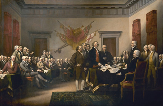
Figure 5.1 The Declaration of Independence by John Turnbull
(Source: http://commons.wikimedia.org/wiki/Category:Public_domain)
In other areas, too, quantitative thinking was beginning to emerge. In design, George Washington instructed the builders of his Mount Vernon estate in colonial America to give stark corners and deliberate shape to the porticoes and columns, a style reflective of his belief in mathematical precision and consistent with themes of the Enlightenment.
Philosophers like Locke and (a bit earlier) Hume, mixed with the politics of Napoleon and those of the church (principally the Catholic Church but also the Church of England), pushed vast change onto society, moving the cultural landscape immeasurably. Their influence on the minds and outlook of ordinary people of the day cannot be overstated. The generations-old overreach of the church was passing. Its decline in influence in the daily lives of ordinary people left room for new thinking.
Hugely influential, too, was the vast rise in literacy, as described in Chapter 4. The number of people who learned to read in this period was prodigious, making this fact alone one of the important societal markers of all time. With their new reading skills, people now had the opportunity to explore new ideas and, with that, to break from staid habits and traditions.
Still, while these forces gave momentum to the quantitative mindset transformation, they did not constitute its most significant impetus. There was an even more powerful influencer: namely, the astonishing developments in mathematics and in probability theory. This is, more than anything else, what spawned the mindset of quantification for an entire populace.
The times were so infused with new mathematical emphasis that, alone, this force could be considered almost primary to the epochal age of reason, self-determination, and mastery of one’s internal environment. It brought the new ability of measuring uncertainty—that is what changed everything. People were now interacting with the world in new and unforeseen ways. They were beginning to employ reason and common sense informed by the ability to quantify the previously dark unknown. This new awareness was slowly, even unconsciously, making its way into people’s daily decision-making. The environment was groomed for people to begin to change their mindset, their worldview—their Weltanschauung—to quantification.
What made the advances in mathematics, statistics, and especially probability theory so prominent was both the sheer volume of new ideas and the absolutely torrential pace at which these developments came. As asserted by one historian of the period: “Statistics shot up like Jack’s beanstalk in the present century. And as fast as the theory [of probability] has developed … the anthropologist must survey a literature so new and so vast that even the expert can scarcely comprehend it” (Newman 1956, 1456).
We saw earlier that Newton principally set the groundwork for all of quantification. However, Newton’s work did not immediately cause people to reform their thinking. As we will see, such a transformation was subtle and largely unrecognized by the populace until it had happened, which took quite a while, at least a hundred years. People did not deliberately set out to adopt quantitative thinking; rather, the environment (in all ways: social, cultural, political, economic, and educational) evolved to such a degree that they were suffused with a quantified mindset without conscious effort.
* * * * * *
Because of the foundation for probability laid down by the three theorems we saw in Chapter 4 (the binomial theorem, the law of large numbers, and the central limit theorem), things really began to take off. One of the early figures in this rapid development was Abraham de Moivre. De Moivre was, first and foremost, a French Huguenot, a member of a relatively small group of Calvinist Protestants who believed that the true route to God was by believing directly in Him, who provided salvation by grace. This was in contrast to the Catholic view that praying through the church leaders and demonstrating good works was the proper avenue to God and salvation. Most especially, the Huguenots were a political threat to the French aristocracy. They became a focus for the French Wars of Religion.
At the time, the slow decline of France was well marked, and the French aristocracy blamed it primarily on the Huguenots and especially their spreading dissent to others. In fact, the French aristocracy’s hatred of Huguenots was so intense that it remained strong even a hundred years after the horrific St. Bartholomew’s Day massacre, when Catherine de Medici ordered French troops to kill all Huguenots and, almost indiscriminately, any sympathizers. In this horrific event and ensuing incidents, somewhere between 40,000 and 100,000 people were killed, with many slaughtered in cold blood. While the massacre actually transpired some time before our story, its effects were long lasting and profound well into the eighteenth century.
The anti-Huguenot sentiment played a large part in shaping de Moivre’s intellectual efforts in mathematics and probability. He saw his energies not solely as advancing mathematics but as an extension of his belief. He said that his intention was to use mathematics to prove the existence of God. Throughout this chapter and Chapter 6, we will see that he was not alone in this perspective—it was a popular pursuit in this time of reason.
But history informs us that de Moivre was not so pure a Huguenot that he eschewed interacting with Catholics and other non-Huguenots. In reality, he was interested in advancing himself politically, which he did through seeking interaction with persons of estimable reputation. He initiated friendships with the most eminent astronomers and mathematicians of his day. His acquaintances included Sir Isaac Newton, Sir Edmond Halley (the English astronomer who precisely predicted the return of the eponymous Halley’s comet), and James Stirling (the Scottish mathematician who proved that Newton’s difficult computations and his invention of modern calculus were correct). August company, to be sure.
Also among de Moivre’s friends were several members of the Bernoulli family. He and Jacob discussed the law of large numbers, and there are accounts that de Moivre expressed to Jacob his admiration for it. Recall, I mentioned in Chapter 4 that Jacob started to describe his theorem (the law of large numbers) in his monumental, but protracted, Ars Conjectandi but that he died before it was complete. Apparently, it fell to his nephew, Nicolaus, to finish the work and bring it to publication.
Nicolaus was also a mathematician, but of nowhere near the stature of his uncle or of de Moivre. Nicolaus, knowing de Moivre’s admiration of Jacob’s work, solicited his help on the task, but, for whatever reason, de Moivre decided against the collaboration. Perhaps this says more about the inadequacy of Nicolaus than anything else; or, possibly, de Moivre was simply too busy at the time. We do not know the reason de Moivre declined the invitation to work with Nicolaus on a project in which he (de Moivre) had expressed passionate interest.
Regardless, de Moivre was fascinated by Jacob Bernoulli’s law of large numbers. He knew that, by applying it to games of chance, he could calculate the odds for a given outcome. Given that he was supporting himself by tutoring in pubs and public houses, this must have been appealing. But de Moivre’s interest in the law and gaming did not stop with tutoring. He pursued it in his academic work, too. By applying Bernoulli’s calculus to the underlying principle of Pascal’s triangle, he demonstrated mathematically how samples of random drawings from a population would distribute themselves around the average value in a predictable manner; namely, the values from the drawn samples were always uniform and symmetric about the average, in a clear demonstration of the central limit theorem.
De Moivre quickly realized that it did not matter what object was being sampled to observe this pattern. It worked equally well with hands in a card game; political attitude; eye color; and most other objects and ideas. This led him to count all kinds of things: the height of people, the age at which they died, the distance between towns, the number of houses in them, the physical features of soldiers, and much more. Seemingly, he counted everything in sight. For each thing he counted, he aggregated his data and then mapped it graphically into what are, effectively, histograms. These enumerated elements became “variables” in his quantitative studies.
To remind you of a histogram, I present one as an example, but I am sure you have seen thousands of them and might even have made them in Excel or another software program. If you are of a certain age, you may even remember creating a histogram with a pencil and graph paper. Just to keep us on common ground, a simple histogram is presented in Figure 5.2. Histograms figure prominently in the development of probability theory.
Figure 5.2 Illustrative histogram
A histogram, like the one in Figure 5.2, displays the possible values of a probability distribution as a series of vertical bars. It is useful to represent graphically the outcome of binomial events (i.e., “either-or,” like coin flips of heads or tails), and histograms are a convenient way to organize data from these observations. Each column presents a frequency count, a discrete value that is less than infinity. Sometimes, these columns are called “bins,” because they capture all values within that group. As a probability distribution, the separate probabilities of each column must sum to one, or 100 percent probability.
In the figure, there are six binomial events: each is a range of temperatures, and they are shown along the horizontal scale, called the x axis. The vertical scale is called the y axis and is a frequency count for how often a particular temperature is observed. In this case, the “Under 30°” temperature was observed five times, and the “31°–40°” temperature was observed twenty-one times. Because there are several binomial events that share a common denominator (in this case, temperature), it is a “binomial distribution.” We will see many examples of the binomial distribution in the remaining chapters. Later on, we will explore how this is actually a probability distribution, rather than just an assemblage of individual events.
Realize, too, that the binomial distribution is but one kind of distribution. There are many. The names for some others are “multinomial distribution,” “multivariate normal distribution,” “chi-square distribution,” “Poisson distribution,” and “Laplace distribution.” Naturally, most of these are technical, and their application is nearly always associated with a given discipline or circumstance, such as medicine, engineering, or business and finance. For the curious, descriptions of lots of them can be found in a comprehensive compendium of distributions offered by Forbes et al. (2011).
De Moivre made thousands of histograms. He noticed that a great many of them were roughly symmetrical, with few instances on the left side, more in the middle, and again few on the right side, as well as the fact that this pattern emerged almost regardless of the variable under his consideration. With some insight, he connected their tops with a line that was itself almost a symmetrical curve. Apparently, he made this little wavy drawing over and over again. For de Moivre, a bright individual with a grasp of higher mathematics, the activity was not child’s play; rather, it was grist for studying the shapes of his diagrams—particularly for defining it mathematically. He focused on exploring “errors” or instances that did not fit his emerging symmetrical curve.
Further, de Moivre appreciated that, by following Bernoulli’s law of large numbers, each curve he had drawn was rather crudely shaped when it comprised only a few points (i.e., distinct observations), but as the number of his data points increased (i.e., more observations), the shape assumed an identifiable form. With a little hand smoothing (formal, statistical smoothing methods had not yet been invented), the rough silhouettes formed a bell shape. By this process, de Moivre had, in effect, invented the bell-shaped curve. Figure 5.3 is de Moivre’s distribution for his “doctrine of chances” from thirty-six random events, with his bell-curve overlay.
Figure 5.3 Illustration of de Moivre’s distribution, from thirty-six random events
(Source: derived from A. de Moivre, The Doctrine of Chances: or, A Method of Calculating the Probabilities of Events in Play)
These observations are specified mathematically by algebraic expressions that can be derived from Pascal’s triangle and are formally solved by the binomial theorem. As is readily apparent, de Moivre’s illustration demonstrates the monumental importance of the theorem.
Today, we refer to de Moivre’s bell shape as the “normal curve.” Of course, he did not call it that, instead labeling his work a “doctrine of chances.” And, significantly, his distribution was not yet specified as a density function (we will see that later on, in Chapter 9), but it did have similar properties: specifically, uniformity and symmetry.
De Moivre published his work in 1718 as The Doctrine of Chances: or, A method of Calculating the Probabilities of Events in Play (de Moivre 1967). The work was also one of the first accountings of a burgeoning probability theory. From its inception, The Doctrine of Chances, with its explanation of de Moivre’s bell shape as the normal curve, has been recognized as an achievement of immense significance. For instance, it was highly praised by an eighteenth-century historian named Isaac Todhunter, who wrote perhaps the first history of probability theory in 1865, titling it A History of the Mathematical Theory of Probability: From the Time of Pascal to That of Laplace. In it, he said: “De Moivre’s Doctrine of Chances formed a treatise on the subject [probability theory], full, clear, and accurate; and it maintained its place as a standard work, at least in England, almost down to our own day” (Todhunter 1865, vii).
Over the following fifty or so years, de Moivre’s drawing of his “doctrine of chances” underwent several transformations, especially in the work of Carl Gauss, before finally settling into the form of the normal curve so familiar today. As another step, Jacob Bernoulli used the word “integral” from calculus terminology for the first time to specify a solution for determining the area under the curve as a density function. Regardless of these later advancements, this is where the familiar bell curve got started: with de Moivre. This was quite a step on the road to quantification.
Even beyond drawing his bell-shaped curve, de Moivre set his observations in tables of values with concomitant probabilities. For example, he invented “life tables,” publishing them in an influential piece titled Annuities upon Lives (de Moivre 1725), which displays a bell-curve distribution of the probability of an individual’s dying before their next birthday. De Moivre actually gave his work a very long full title: Annuities upon Lives: or, The Valuation of Annuities upon any number of Lives; as also, of Reversions. To which is added, An Appendix concerning the Expectations of Life, and Probabilities of Survivorship. Its breadth of coverage and sustained importance is described in the book’s appendix, which was written by an anonymous author, who says,
De Moivre’s contribution to annuities lies not in his evaluation of the demographic facts then known but in his derivation of formulas for annuities based on a postulated law of mortality and constant rates of interest on money. Here one finds the treatment of joint annuities on several lives, the inheritance of annuities, problems about the fair division of the costs of a tontine, and other contracts in which both age and interest on capital are relevant. This mathematics became a standard part of all subsequent commercial applications in England. (de Moivre 1725, DSB IX: 454)
By the way, a “tontine” is a specialized investment plan in which individuals buy shares in a monetary investment (like an equity fund or real estate parcel) to form a pool of investors, who receive an annuity that increases whenever one of the other participants dies. De Moivre uses statistics to illustrate his examples that he had garnered from Halley’s work in the 1690s. He computed tables from his bell-shaped curves to show longevity and rate of return. Today, de Moivre’s tables are still used, commonly in economics and in the insurance industry but also by governmental agencies and, doubtless, others. We now call his life tables “actuarial tables.” Across the globe, students today learn these features for investment based on—you guessed it—de Moivre’s Annuities upon Lives.
* * * * * *
As an ever-inventive mathematician, de Moivre did not stop at simply mapping his distributions, even though that was a significant invention in itself. He extended his work to compute yet another statistical measure, this one of dispersion about (i.e., above and below) the mean: the standard deviation. He refers to this concept as a “theory of error”; the term “standard deviation” did not come into use until much later. As we have seen already, others (notably Galileo) had previously observed variations about the mean, and even the fact of its symmetry. But they did not carry the work forward, instead merely attributing it to “error in observations.” De Moivre, however, formalized the variations into a systematic measure of dispersion, a measure that could itself be calculated and studied.
Today, students worldwide in beginning statistics classes and elsewhere memorize de Moivre’s formula and learn how the standard deviation operates. For curiosity only, I show the formula as used today for the “population standard deviation” (there is a slight adjustment to it when the intent is to calculate it for the “sample”). The Greek letter sigma (σ) is universally accepted as the symbol for standard deviation in a population. (In a sample, it is just abbreviated as SD, and µ represents the population mean value.) It is
De Moivre made his original calculation a function of the variance notion for any “standard normal deviate” (or “z-score”), which has the advantage of applying to any variable expressed in standardized form. This form also allows for specific expectations about the full range of a variable, which we discuss momentarily. Both forms lead to the same result; the difference is that the one given above is statistical in nature, implying that it is directed at a practical utility (as in a research scenario), while de Moivre’s formula is more mathematical, and as a function implies that an algebraic or calculus proof is to follow. Actually, de Moivre developed his idea into a theorem about the variance of a distribution. Hence, this form is called “de Moivre’s theorem.” It is
De Moivre then went on to provide the missing calculus proof. This was a huge step in probability theory because now, not only was the mean useful in understanding a phenomenon, but so too was its variation.
By formalizing the standard deviation with a calculus proof, de Moivre provided a mathematical rationale to explain the fact that, in a perfectly symmetrical distribution, approximately 68 percent of the observations fall within one standard deviation of the mean of all the observations. By extrapolation (also, more technically and exactly by integration), more than 95 percent of observations fall within two standard deviations or, similarly, any other point along the distribution.
In a syntactical sense, the standard deviation is the average error, or, in general terms, the average amount by which the observed values will deviate about a distribution’s mean. Figure 5.4 shows de Moivre’s distribution with standard deviations. As shown, the distribution represents a population (rather than a sample) whose mean is represented by µ and the standard deviation by σ, as we saw earlier.
Figure 5.4 Illustration of de Moivre’s distribution with centered mean and standard deviations
(Source: derived from A. de Moivre, The Doctrine of Chances: or, A Method of Calculating the Probabilities of Events in Play)
As we just saw, de Moivre developed his notion into a theorem that derives from the central limit theorem. Actually, it is a special case of Laplace’s work wherein the normal distribution is approximately the same shape as and has characteristics of the binomial.
De Moivre wanted to prove his theorem and used coin tosses to illustrate random events. Being a practical person, he literally tossed a coin 3,600 times (!), following Bernoulli’s trials, and ultimately discovered that the probability distribution from such a tiring experiment would indeed be a bell shape. He described this work in the second edition of his by-then-famous Doctrine of Chances and gave credit to his forerunners: Newton, Bernoulli, and especially Laplace. As his work is an important application of the central limit theorem, today we give credit to both men, calling it the “de Moivre–Laplace theorem.” It is a special case of the more general central limit theorem.
When introducing de Moivre, I emphasized his French Huguenot perspective, as it was so important to him. Recall that his primary interest in studying phenomenon was not so much as a theoretical mathematician but as a means to advance his Protestant beliefs and that he was actually trying to prove with mathematics the true existence of God. In philosophy, he worked from an “originalist” perspective. Reflecting the philosophical milieu of his time and his deep Protestant faith, de Moivre saw a grand design in the universality of the bell curve, which he attributed to God. Using the stilted composition of the day, he explained his idea by saying,
Altho’ Chance produces Irregularities, still the Odds will be infinitely great, that in the process of Time, those Irregularities will bear no proportion to the recurreney of that Order which naturally results from ORIGINAL DESIGN. (de Moivre (1738) 1967, 251)
In this quote, de Moivre reveals two things about himself. First, he believes that there is an order to all things, far beyond random happenings (chance “irregularities”), which is revealed in many trials over the course of time (“process of Time” and “recurrency”). And second, this order comes from God as original design. Note that, concerning the first point, symmetry exists in nature and, in man’s mathematical inventions, cannot be denied.
The proposition, then, is not of the veracity of symmetry (de Moivre’s first point) but of an origin for it (i.e., divine or naturally occurring), his second point. It is clear where de Moivre stands. Obviously, the bell-shaped curve is a tantalizing hint of original design for all kinds of variables.
To be sure, de Moivre’s principal argument was ontological in the tradition of Western Christianity and specifically followed the ideas of René Descartes. Descartes, himself both a mathematician and a philosopher (he is often considered the “father of modern Western philosophy”), famously put forth his “proof” for God, following the logic that if the greatest possible being exists in the mind, it must also exist in reality. Descartes developed his ideas in a wealth of writings that have come to form the basis for debate about God’s existence.
You likely know that the debate continues to this day, sometimes titled as “original causes” or “first causes.” (A modern offshoot to this thinking is “intelligent design” or “original design.”) We will see this debate resurface in the work of Bayes and Laplace, where it is integrated into probability theory as the existence of God being a likely event. With de Moivre, however, it shows the strong influence of newer thinking on Christianity—thinking that allows a quantitative approach to theological study, even to the most foundational of theological questions, is there a God?
This question has spawned an entire genre of study, in mathematics, in religion, and in philosophy, where it occupies much of the scholarship in ontology and epistemology. There are academic journals, university courses, conferences, and countless Sunday sermons devoted to the examination and debate of original design. It is an interesting topic to explore, and one that gives light to how deep the notion of quantification goes into our very souls, including our conception of the ultimate Truth: the existence of God. Of course, humankind has pursued this question since the beginning of time.
The notion of quantification in nature and its being God ordained was not only present in de Moivre’s bell curve; it was moving within the broader society as well. For instance, the English poet and philosopher Alexander Pope, writing at this same time in his famous Essay on Man, sought to “vindicate the ways of God to Man,” a variation on Milton’s message in Paradise Lost to “justify the ways of God to Man” (Mack 1985). Written in heroic couplet (a mathematics-based poetic meter popularized by Pope in the poem), it attempts to show that “natural laws” (i.e., symmetry in nature) consider the universe as a whole and a perfect work of God. This was a popular sentiment at the time.
To our purpose, it also brings quantification to literary circles, a sphere with influence far beyond the rarefied world of mathematicians. Add to this mix the influence of religion by de Moivre, Descartes, and Pope. In their collection, we are witnessing the spread of quantification to ever more spheres of human thought and involvement. Thus, its influence is growing less obtuse, and more concrete, with respect to the daily lives of ordinary people.
With religion as his foremost thought, considering the context of the times (with still strong anti-Huguenot sentiment left over from the French Wars of Religion), life was not always easy for de Moivre. When de Moivre was just eighteen, King Louis XIV revoked the Edict of Nantes, a decree of religious tolerance granting Protestants equality with Catholics. The edict was originally intended to placate the Huguenots within France, but their obstinacy continued, as did their anti-aristocracy message. Eventually, the French government, and particularly the ruling aristocracy, decided they had had enough. The religious decree was cancelled. With no decree to protect his religious freedom, de Moivre was asked to swear his allegiance to the king, a requirement for all French citizens. But, being staunchly Protestant, he refused, and because of this, he was jailed for two years. Upon release, he moved to England (along with thousands of other early Protestants who were also persecuted by the French), where he continued his work in mathematics. It was there he met Newton and the others.
De Moivre had other setbacks, too. Despite his friendships with many important people, and notwithstanding his prodigious achievements, he seems to have been a genuinely unhappy person. Bernstein (1998) reports that de Moivre was introspective and bitter about his ever-languishing career prospect of being a university professor. More than anything, de Moivre wanted to be a professor at one of the better-known universities, but it was not to be. For most of his adult life, he unsuccessfully applied for one academic professorship after another. Needing a living, he was forced to support himself mainly by tutoring young students. Sadly, he died at the age of eighty-seven, blind and poor.
One legend about de Moivre (some biographers dispute its authenticity, but it is widely reported) is that, in later life, he began sleeping more, adding about five minutes additional sleep each night. Knowing this, he reasoned that when the additional sleep time added up to his sleeping twenty-four hours, he would be dead! From this, he computed the date on which he would die: November 27, 1754, which turned out to be his dying day. We do not know whether de Moivre took comfort in his accuracy.
* * * * * *
From here on out, this kind of bell-shaped curve will reappear in our story regularly because it is basic to quantifying data and essential to its harmonizing place in our lives. To us, the famous curve looks ordinary, and we can imagine all sorts of instances where it could apply: grades or achievement test scores in school; height or weight; ages for mortality; incidences of morbidity; income across populations; and so forth. Readers may remember a popular book in the 1990s titled The Bell Curve, written by the respected Harvard professors Richard Herrnstein (a psychologist) and Charles Murray (a political scientist) (Herrnstein and Murray 1994). Despite their solid scholarship, the book’s thesis was hugely controversial because they touched the nerve of differences in IQ. But controversy aside, for modern people so heavily steeped in a quantified world, there was no question about the title: everyone—from scholars who calculate it with integration as a density function to the illiterate individual who cannot cipher the caption—recognizes what a “bell curve” is. Anyone who sees one knows what it is. This is quantification as our worldview today.
For historical perspective, realize that the time of de Moivre was the late eighteenth century, when it was not common to count things and then arrange the values in a distribution. There was no quantitative mindset. The bell curve had not been formalized, and most folks did not even know about it. Had Herrnstein and Murray’s book been published then, its title would have been a mystery. This shows how far quantification has come.
In de Moivre’s time, however, most people simply had no notion or perception of a bell-shaped distribution or, more broadly, of measuring uncertainty. They lived in a world of reacting to events only after they had happened. Decisions were made by whim, habit, or tradition. Everything happened to people unexpectedly, with little awareness that soon both everyday and not-so-ordinary future events would be predicted or forecast. But with Bernoulli, Mozart, Ben Franklin, and now Abraham de Moivre on the scene, things were changing—subtly and slowly, to be sure, but dramatically nonetheless. The influences for bringing quantitative thinking to the fore for everyone were now in place.
From Dr. Johnson’s poetic insight on observation through the awesome beauty of the nautilus shell to the mathematical and statistical discoveries and inventions that form the foundations of probability, a new quantitative Weltanschauung (worldview) was beginning. The seeds were sown—and more importantly, they were beginning to grow in people to become a soon-to-be new perspective on everything.
* * * * * *
In order to clearly understand upcoming developments, a bit of specialized vocabulary is needed. Specifically, we look at three terms: probability, odds, and likelihood. These terms will follow us throughout this book, so beginning with a clear understanding of their meaning is important. These interrelated terms comprise nearly the whole of probability theory because they are the object of its techniques. In other words, when a statistician employs one of the methods of probability theory (we explore some of them in the next several chapters), it is for the purpose of estimating odds, probability, or likelihood. As I explain these concepts, a few other vocabulary words will pop up, but their definitions are fairly obvious, and I doubt you will get lost.
Aristotle said, “The probable is that which happens often.” Simply but significantly, probability is the chance of something happening, which is labeled an “event” in probability theory. An event is either a planned circumstance in research (wherein we set up an experiment of some kind, such as when examining a new medical drug to determine whether it is safe for general use) or a natural phenomenon (such as gender, height, ethnic heritage, and the like). Realize that events are constrained to just these contexts within statistics and probability theory, so not everything is a statistically relevant “event.” It would be silly to think of each nanosecond of our lives as an event. However, in the probability theory context, every event leads to an outcome, although at the beginning we do not know what that outcome will be. Flipping a coin as a simple experiment to see which side lands up is an event, but initially we do not know the outcome (whether heads or tails)—only that there will be an outcome. Hence, by definition, events have outcomes. With the coin toss, there are two outcomes: heads and tails. In probability theory, this is noted as (0, 1) (read: zero, one). If we look for a given binomial outcome, the result is called “success” or “failure.”
Realize that the number of possible outcomes will vary with each experiment or circumstance. It can be two, just a few (as is the case for, say, the number of children in a typical household), or several (such as the number of insect pests that feed on a given plant); or, of course, the number of outcomes can grow to millions and millions (as with stars or lottery numbers).
In exact probability applications, the theoretical domain of all possible outcomes is called the “sampling space.” This is as far as we go technically with this idea, but there is much more to it.
Odds, our next term, is the expectation of a given outcome being the observed result of the experiment or natural phenomenon. Thus, odds represent the probability of success in outcome. They are calculated as the ratio between the number of successful outcomes in an event and the number of possible outcomes. To calculate odds, simply divide the former value by the latter. When predicting a given face value on a die, for example, there is one successful outcome and five unsuccessful outcomes, a ratio of one in six (the total number of sides), written as 1:6. The odds are calculated as 1 divided by 6, or 0.1666, about 17 percent. With a lottery, the odds may be 1:240,000,000 (one in 240 million) or some such. As is evident by now, in statistics, odds and probability are not synonyms.
Odds change, but not the probability of success versus failure. All instances of probability are restricted to the interval (0, 1). Think of how many times this applies to your life decisions, big and small, for success versus failure, even when the possible outcomes are many: Did I pick the right investments for my retirement account?, Will holding greater inventory in my business result in faster customer fulfillment?, and so forth. The possible outcomes for each event are many … and can be infinite, in fact, in the sampling space. But observing a given outcome is still a probability of (0, 1).
Our final term in this vocabulary of probability theory is likelihood. In statistics and probability theory, this term is used technically and means the probability of a given sample being randomly drawn from the parameters (mathematical limits) of a population. In calculations, the term “likelihood” is used rather than “odds,” because of its reference to population parameters. The most probable outcome (greatest likelihood) from among all the possibilities (in the sampling space) is called the “maximum likelihood.” Often, we wish to calculate the maximum likelihood; we do so by a process called “maximum likelihood estimation,” abbreviated as MLE. Given that the MLE equation is a function of various kinds of information (in particular, “conditional probabilities,” as described below), it is called a “maximum likelihood function.”
So now we have our three terms: “probability,” “odds,” and “likelihood.” In most scientific contexts, it is important to use them correctly. Of course, when using these terms in popular speech, things are not so fussy. Among friends, they are just words that convey approximately the same meaning.