CHAPTER 9
Here, at last, is our Carl Gauss: the Princeps mathematicorum, Latin for “the foremost of mathematicians.” His full name was Johann Carl Friedrich Gauss, but he is commonly known as either Carl Gauss or, using his original first name, Friedrich Gauss. Today, he ranks among the greatest mathematicians that the world has ever known, along with Archimedes, Isaac Newton, and Leonhard Euler. Quite remarkable.
Even his signature displays a certain eminence, as seen in Figure 9.1. A noted biographer of Gauss describes his handwriting as “beautifully clear” (quoted in Bell 1956, 339). His signature and handwriting are a kind of metaphor for his clarity in composition and lucidity in thought: carefully considered and with attention to detail, not hurried.
Figure 9.1 Carl Fredrick Gauss’s signature
(Source: http://commons.wikimedia.org/wiki/Category:Public_domain)
Carl Gauss (his image is seen in Figure 9.2) was, quite simply, a man of amazing accomplishment, and he was pivotal in advancing quantification, both through his numerous mathematical discoveries and for his spreading quantification to an ever-widening audience. He was a man of unquenchable curiosity. Although he worked almost exclusively in mathematics, the breadth and scope of his quantitative achievements advanced astronomy; calculus; statistics and probability theory; number theory; algebra including matrix theory; geometry; geodesy; geophysics; magnetism; mechanics; and even optics—quite a list. It all represents a range of accomplishment that is simply astounding for a single person. One noted historian of mathematics summed up Gauss’s career by stating, “He lives everywhere in mathematics” (quoted in Newman 1956, 339).But he had a special interest in number theory. He said, “Mathematics is the Queen of the Sciences, and Number Theory the Queen of Mathematics” (quoted in Bell 1986, xv).
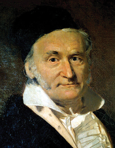
Figure 9.2 Image of Carl Friedrich Gauss
(Source: http://commons.wikimedia.org/wiki/Category:Public_domain)
Gauss loved mathematics to the point of obsession. Beginning at a young age and continuing until his dying day, mathematics was his life, occupying his every thought. When informed that his years-long-ailing wife was dying, he is reported to have said, “Ask her to wait a moment, I am almost done” (quoted in Bell 1986, 201). Don’t be too quick to judge him, however. In truth, he was a compassionate man who spent many years as the care giver to his mother and then to both of his wives during their respective long-term illnesses. Regardless, for Gauss, mathematics was everything.
Even at a very young age, Gauss was more than just good at mathematics—he was a child prodigy. The tales of his amazing feats in mathematics while he was still a juvenile are the stuff of legend. His childhood years are recounted in many stories; the full truth is often unverified, but the amazing tales are commonly repeated. His documented accomplishments, however, are so numerous and impressive that the anecdotes are certainly believable. By any account, his genius was on par with some of the greatest, such as Pascal (who wrote a treatise on vibration at age nine, putting its proof on a wall with a lump of coal), Mozart (who composed a full symphony at age five), Chopin (who was composing at age six), or William Sidis (the youngest person to enter Harvard, at age eleven).
There are many stories of his photographic memory, such as being able to recite long passages from books he had read only a single time, years previously. He remembered the name of everyone he met, even if only in passing, and could recall verbatim their exact conversation. We saw earlier that Gauss developed one of the most important mathematical inventions of all time, his method of least squares, when only eighteen years old. Further, he later provided the calculus proof of this method when others could not. He developed a special instance of reaching solution in some kinds of calculus integration called a “Gaussian quadrature,” and a particularly useful form called the “Gauss–Hermite quadrature” wherein the values for integrals can be approximated. For persons working with calculus to solve all kinds of real-world problems (e.g., in engineering), these Gaussian methods are of enormous practical value.
A popular story is that, at age three, he noted an error in his father’s reckoning and, meaning to be helpful, pointed it out to him. Instead of showing amazement or appreciation, however, the elder Gauss who was an uneducated, poor laborer, berated young Carl harshly. Apparently, he didn’t like being upstaged by his own son. Throughout Carl’s childhood, his father resented the boy’s aptitude for mathematics and his general intelligence and often showed the sensitive child a cruel and inhibiting hand. His mother, however, presented a kinder approach in raising Carl and saw to it that he got a good education, despite their poverty.
By fortune, the Duke of Brunswick, Carl Wilhelm Ferdinand, learned of the young prodigy; and, upon seeing young Carl’s genius, the duke was so impressed that he assumed patronage, financially supporting Gauss’s university education and even offering assistance for some years after graduation. The duke continued to support Gauss until his own death by gunshot. Their meeting was a happy accident—one that changed the course of history and whose influence lives on in us through our quantified outlook.
A popular anecdote of young Gauss’s feats includes his mother. She was illiterate and did not record his birthday. When he asked her about it, she could only remember that it was on a Wednesday, eight days before the Feast of the Ascension (also known as Holy Thursday, it commemorates Christ’s ascension into heaven three days after the crucifixion). Gauss knew that the Christian holiday occurs 39 days after Easter; but, as readers likely know, Easter is not on a fixed date but calculated anew each year: it is the first Sunday after the fourteenth day of the lunar month that falls on or after the vernal equinox, which is usually around March 21. Gauss calculated the date for the Feast of the Ascension for his birth year—and, from there, he figured out his own birthday: April 30, 1777. One hopes a cake with the correct number of candles on it was then presented to him each year thereafter.
Not stopping with calculating his own birthday, Gauss went on to derive formulas for finding any date, past or future. Gauss’s annular formulas are still used today—if you have a smartphone, it probably has the formulas imbedded in a chip. Albert Einstein is said to have remarked that not only was Gauss the only one who could have come up with these formulas, he was the only one who would have thought that it would be possible to come up with them in the first place (Schocken 2015).
His scholarship at school was legendary. Once, when he was eight, his primary school teacher asked the class to add the numbers 1 to 100 (“What is the sum of the first one hundred whole numbers?”). The students dutifully set out to do the addition, but Gauss reasoned that using a formula would be faster. He split the numbers into two groups: 1 to 50 and 51 to 100. When he added the first digit from Group 1 to the last of Group 2, it summed to 101. Next, when he added the second digit from Group 1 (“2”) to the penultimate number in Group 2 (“99”), it also summed to 101, and so on for each pair. He reasoned that adding 1 to each successive number in the first group and subtracting 1 from each number in the second group would give him 50 pairs of 101, which multiplies to the correct answer: 5,050; in other words, the equation 50 × 101 = 5,050. What’s particularly interesting is the elegance of Gauss’s formula: 1 + 2 + · · · + n = n (n + 1)/2. Remember, he was only eight years old!
Gauss completed grammar school early and, at just fifteen years old, entered Collegium Carolinum (now renamed University of Braunschweig–Institute of Technology), intending to study languages, but he soon came to pursue mathematics. He graduated three years later with a degree in that field. Thereafter, he transferred to the University of Göttingen to further his studies. He returned to his hometown of Brunswick and completed his doctoral studies at Helmstedt University in 1799. In his dissertation, Gauss provided a proof for the so-called fundamental theorem of algebra, a difficult complex of numerical relationships, whose proof had eluded many professional mathematicians. (For mathematically curious readers, the full proof can be found at various online sites (e.g., see Cain 2017)). Gauss did this difficult work when he was barely twenty-two years of age.
Many of Gauss’s discoveries came early, some while he was still a teenager. When just fifteen years old, he grew interested in finding the answer to a problem that had eluded even the best mathematicians of the day: finding a pattern in an array of apparently random prime numbers. After some study, he realized that, given these numbers increase by ten, the probability of a next prime reduces by a factor of approximately 2. He had found a hidden pattern. However, his pattern was not exact and thus he could not produce a proof, something Gauss believed necessary for completion. Because of this, he kept his solution secret for much of his life. Since then, however, others have given Gauss credit for coming closest to a solution.
In another problem, when he was just nineteen years old, Gauss demonstrated that a regular polygon of seventeen sides can be constructed by a ruler and compass alone. This was a major discovery in the field of mathematics, as construction problems of this type had baffled mathematicians for centuries. Astonishing work for a student—but then, remember this student was Carl Gauss! We are, indeed, grateful to the duke for ensuring that so deserving a young genius as Gauss got the education necessary to take advantage of his talents.
One of Gauss’s most important quantitative advances was in number theory, an achievement he codified in 1798 but did not publish until two years later when he was twenty-one, as part of his magnum opus Disquisitiones arithmeticae. (Readers will recall that we saw this book in Chapter 7 when we were discussing Gauss’s version of the method of least squares, and its comparison to Legendre’s version.) It has been said that this book is as important to number theory as Euclid’s Elements of Geometry (1491, Euclid et al. 2010) was to geometry. Both works are foundational, not only to their respective fields but to mathematics and philosophy generally. Some of his other achievements are the Gauss unit (in magnetic field theory), the Gauss–Markov theorem, Gauss quadrature, and Gaussian correlational inequality.
Later in the same year that Disquisitiones arithmeticae appeared, Gauss published Theoria motus corporum coelestium (Theory of Motion of the Celestial Bodies), which is his most important work on applied mathematics (Gauss 1871). His theory introduced the Gaussian gravitational constant. It remains today a cornerstone of astronomical computation. Every NASA mathematician, engineer, and physicist knows about this constant and uses it in their calculations.
Throughout his life, Gauss was awarded numerous prizes, including the prestigious Lalande Prize for his contributions to astronomy, the Danish Academy of Sciences for his study of angle-preserving maps, and the admired Copley Medal for his inventions in magnetism. There are more than one hundred theorems, processes, laws, and proofs named after Carl Gauss, to say nothing of all the other things named after him, showing the truly dizzying scope of his achievements in astronomy, physics, probability theory, statistics, calculus, and other applied and theoretical mathematics. The professional society International Mathematical Union convenes a mathematical congress once every four years to discuss achievement in the mathematical sciences. At the opening ceremony, it awards the Carl Friedrich Gauss Prize for Applications of Mathematics in his honor. It is one of the most respected awards that the field has to offer, on par with the ultra-elite Fields Medal in Mathematics (also awarded only once every four years). (Notably, there is no mathematics category in the annual Nobel prizes.)
In addition, Gauss was offered several other awards and even professorships at important universities (including Berlin University, around 1817), but he routinely declined them because he was loath to leave his hometown of Göttingen. The affinity he had for his native town, in the pressures of so strenuous and exacting a career, is a bit of a surprise, but he had his reasons. His mother fell ill, and he took her into his house to care for her throughout her remaining years, more than twenty. Later, in succession, both his first and his second wives also became infirm for many years, and he cared for them, too. So, despite the earlier quote, it seems Gauss was a sensitive caregiver.
As one can imagine, Gauss’s fame was worldwide, particularly in his homeland of Germany, but he was also known throughout the Continent and even into Eurasia. He eschewed the notoriety, however, preferring to work in the relative inconspicuousness of his study. One story about his renown is that, during the Napoleonic Wars of 1803–15, as Napoleon’s troops were approaching Gauss’s hometown, Napoleon ordered them to go around Göttingen and spare it because “the greatest mathematician of all time is living there” (quoted in Bernstein 1998, 168). Certainly, Napoleon made the right call that time.
Perhaps a more significant recognition of Gauss’s genius and his accomplishments, however, was paid by Laplace, the acclaimed French Newton. After the Napoleonic Wars, the victorious French demanded money from their vanquished foes, asking the enormous sum of 2,000 francs from Gauss. Living on the modest means of a university professor, Gauss simply could not afford that amount; plus, he simply objected to the French demand and refused to pay it. Laplace, a man of relative wealth, paid Gauss’s fine, saying that he did so because Gauss was “the greatest mathematician in the world” (quoted in Bell 1986, 242). Coming from the eminent Laplace, this was a supreme compliment.
Gauss, typical of his careful nature and thoroughness, often did not publish his findings as he worked on a problem, sometimes waiting years before making his work public. He frequently kept his ideas to himself and returned to a given notion many times over the years, almost always changing and adding to it before finally releasing it. His motto was Ut nihil amplius desiderandum relictum sit (“that nothing further remains to be done”). When he did publish one of his ideas, he was elegant and detailed in his explanations, always including a thorough proof. Many times, he gave several proofs, and more than once he even offered explanation of why no additional proofs were possible.
All told, Gauss published more than 155 meticulously researched and written papers. There are several modern collections of them. One of the largest collections of his publications and personal papers is held at the Cammie G. Henry Research Center at Northwestern State University of Louisiana, thanks to the thirty-year collection effort of a determined professor (see Louisiana 2018). Also, the Gauss Society at the University of Göttingen is active in commemorating his work, and they maintain a collection of Internet links to Gauss’s works and life (see Gauss Society 2018).
Gauss was married twice. With his first wife, he had three children. She passed away after a long illness. He then married her best friend and had three more children before her demise, also after a lengthy illness. He spent most of his adult years caring for his mother and then his wives. In older age, he grew increasingly infirm himself, and, in the last years of his life, his daughter Theresa cared for him. He died at age seventy-seven, in 1855.
Now, we turn to describing a few relevant terms, and then specifically to how this remarkable man’s accomplishments advanced the story of quantification.
* * * * * *
We reach a point in our story where it is necessary to employ some terms—not too technical, but it is important we use them correctly, to avoid confusion. Earlier (at the end of Chapter 5), we saw the definitions for “probability,” “odds,” and “likelihood.” Here, we expand this list of terms to include sample space and random variable and, specifically, two types of random variables: discrete and continuous.
“Sample space” is the number of possibilities in an experiment or research context. For example, if the experiment involves rolling a single die, the sampling space is just 1, 2, 3, 4, 5, and 6: all the possible outcomes. Of course, typically the sampling space is much larger. Say, an experiment focuses on an adult’s weight—then the sampling space is all the possible weights (usually within reason): say, from 80 to 500 pounds. While possible weights are above and below these limits, such extremes are so rare as to be ignored. In some experiments, there may be more than one sampling space, such as when drawing cards from a standard fifty-two-card deck. One sampling space could be any card at all, while another sample space may be restricted to face cards only. It is defined by the researcher.
A “random variable” is not quite just any number at all. Rather, a random variable quantifies an outcome. For example, if the variable is rainfall within the last twenty-four hours, then a random variable is the amount of measured rainfall. It could be any number that falls within the sampling space (that is reasonable), say, rainfall from 0 to 50 inches. This means, too that a random variable has a probability distribution. We saw this earlier in Chapter 5, when looking at a histogram. As we know from the central limit theorem, with more trials (i.e., samples), this distribution will tend toward the normal (bell) shape.
Variables themselves can be either “discrete” or “continuous.” A discrete random variable is one which may be any distinct value within the sampling space, such as 0, 1, or 102. A continuous random variable is one which can be any of an infinite number of possible values. These are usually measurements, such as an achievement test score, the time taken to run a marathon, or height or weight. While (in theory) these values can be ±∞, it is usual to truncate the range to just reasonable values. Also, the numbers are limited by the scale on the dependent-variable measuring instrument. For example, if a test score is measured in whole numbers, then a fractional value would not be considered in the sample space.
* * * * * *
Now, with this background, we return to describing the accomplishments of the remarkable Gauss, as they contribute to quantification. The noted dispute with Legendre over authorship of the method of least squares has a more confused—and confusing—context than simply a debate over “who got there first.” Recall, I described a simple version of the procedure in Chapter 7 and identified it as OLS (ordinary least squares) regression. Legendre claimed the invention as his own, and it is indisputable that he published a version of the method first. But Legendre’s original description was relatively elementary, proffering only an algebraic explanation of adding up residual values of the difference between the observed data and the closest point on the regression line. He did not provide a rigorous rationale, nor did he give a calculus proof, usual requirements for a newly invented procedure. What he presented was important, but not sophisticated in the form given.
Further, at the time of its publication, Legendre did not seem to give it much weight, as he included it only as part of an appendix to another publication, and his text was limited to just the simple explanation and one example. It was not until after Gauss had put forth his much more sophisticated version that Legendre very publicly claimed authorship.
Gauss did not dispute that Legendre had published a summing procedure first, but he claimed that he had, in fact, invented the method of least squares years ahead of Legendre. To buttress his assertion, he produced earlier papers where he had employed it several times without mentioning it as a new procedure. He said that the Legendre version was so simple that he had used it for years, as almost routine.
In the end, Gauss got the better of the dispute, both rhetorically and in technical achievement. As for the argument itself, it was mostly carried out in a series of letters to others. Recall that he expressed surprise that Legendre was claiming credit for something Gauss saw as so straightforward that it was barely even worth mentioning. This is scarcely the attitude of a gentleman with the personal empathy he showed in caring for his ailing mother and his infirm wives. But then, Legendre was not such a good guy either, wanting all the credit for something that was an accumulated achievement and making a fuss only after Gauss presented his more sophisticated version. Gauss, as we now realize, invented the generalized method with a more rigorous rationale and a calculus proof. Legendre’s accomplishment is now viewed as very useful, but as just one application of the method of least squares.
Recall, too, that this dispute with not the first between the men. Earlier, Legendre tried unsuccessfully to address a complex problem of astronomy but eventually abandoned his effort. But Gauss was only nineteen years old when he successfully solved it. His work is now adopted as the law of quadratic reciprocity.
In terms of today’s version of the method of least squares, Gauss defined the sample space of a combination of observations as a density function, requiring estimation by calculus. He thereby extended the one-case example of Legendre, allowing it to be appropriately used to estimate population parameters. This step is what distinguishes Gauss’s method from the simple summing procedure of Legendre. I explain the notion of a “density function” momentarily, after completing this bit of history.
As a consequence, thanks to Gauss, the method can be made broadly generalizable and may be used in many scientific contexts. Today, his rationale and proof are the accepted versions. This was a major advance for statistics and immeasurably advances quantification in our storyline.
Gauss demonstrated his least squares method by using it to solve a now-famous problem in astronomy called the “Ceres estimation.” On January 1, 1801, the Italian astronomer Giuseppe Piazzi discovered a new and important asteroid he named Ceres. He tried to figure out its orbit, tracking it for forty days before he could no longer see it because of the glare of the sun. He wanted to know where Ceres would emerge from behind the sun to be seen again. But he did not know how to calculate this—nor did other astronomers. At the time, it was a well-known mathematical Gordian knot. Actually, this particular problem was part of a larger unknown for determining the orbits of celestial bodies.
The problem was vexing to all astronomers and physicists until Gauss, at just twenty-four years of age, applied his version of the method of least squares. Using only three of Piazzi’s observations, he correctly calculated the when and where of Ceres’s reemergence. Gauss published his solution in his Theory of the Combination of Observations Least Subject to Error (Gauss and Stewart 1995). Fortunately for us, Gauss’s original sketches of his work on the problem survive today at the University of Göttingen, shown in Figure 9.3.
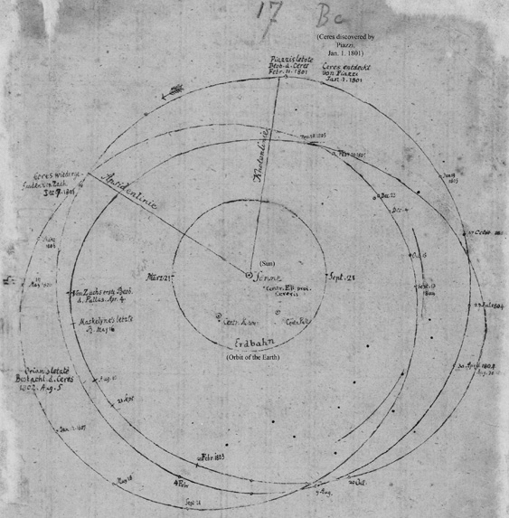
Figure 9.3 Gauss’s sketch of Ceres’s path
(Courtesy of SUB Göttingen. Cod. Ms. Gauß Handbuch 4, p. 1)
Young Gauss’s calculation was an amazing mathematical feat. His reputation was set by it, and, just as important, he established the method of least squares as verifiable. There are several good reads (although some are mathematical in nature) of how Gauss determined the orbit of Ceres (see Teets and Whitehead 1999, Le Corvec et al. 2007). One especially interesting historical record is by Johann Pfaff in his Programma inaugurale in quo peculiarem differentialia investigandi rationem ex theoria functionum deducit, a work in which Gauss scribbled notes of his proof—maybe for the first time—on a back page and signed the frontispiece. Pfaff was also Gauss’s dissertation advisor. A recent first printing of this work was made available for sale at an initial auction price of $75,000, the size of which was attributed mostly to the book’s inclusion of Gauss’s handwritten notes and signature.
In determining the orbit of Ceres, Gauss realized that an underlying harmonic motion that helped to explain the changes observed in the positions of the planets was also useful in estimating large distances on the earth. From this observation, he began his work on geodesy, the science of determining the distance between two points that are far apart, such as the distance between cities or between continents, where the curvature of the earth must also be considered. During his life, he was quite well known for this pursuit. He was commissioned by George IV of England to survey the Kingdom of Hannover, a hilly area whose dimensions had previously been unknown. He set about this work by first making a remarkable invention: the heliotrope. This device is a sort of specialized small telescope that measures angles on the land topography from rays of sunlight. From this, distances can be estimated with reasonable accuracy. While small in comparison to an observatory’s telescope, the heliotrope stood nearly four feet tall. There are stories of various measurements across the countryside taken for the first time using Gauss’s equipment. A picture of his invention is shown in Figure 9.4.
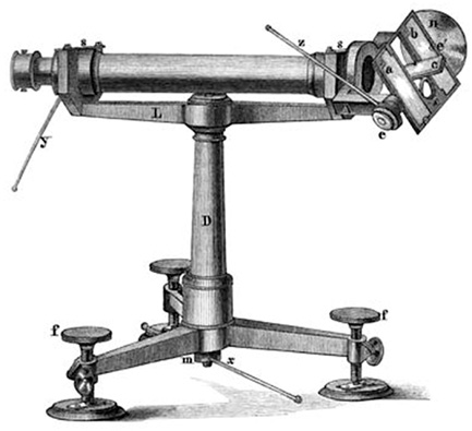
Figure 9.4 Gauss’s heliotrope, about 1822
(Source: http://commons.wikimedia.org/wiki/Category:Public_domain)
In particular, the specific achievement of accurate measurement of long distance brings quantification closer than ever to the daily lives of ordinary people. For example, people could now anticipate how long it would take them to travel between cities. This seemingly ordinary reckoning brought common distances into the daily lives of folks, contributing to quantification as a mindset.
* * * * * *
Up to this point, we have traced the development of the normal distribution (and especially its bell shape), as seen through the work of Laplace and others. They were captivated by the fact that this distribution occurs for everything measurable everywhere in nature (e.g., height, weight, test scores, opinions, rainfall, the size of pumpkins). But, their efforts were not merely to satisfy a simple curiosity. They realized an empirical interpretation, too. Such a scientific realization was advanced by de Moivre, who explained through the central limit theorem why this distribution occurs so regularly in nature. But, these efforts, while significant, were constrained to mere frequency counts, and development of the normal distribution had seemingly come to a standstill.
Then, Gauss, with his characteristic ingenuity and persistence on a problem, realized that the bell shape can be a function rooted in probability. And that this probability function need not be limited to just the bell-shaped distribution. Any distribution, regardless of its resultant shape, can be a function of probability.
By this reasoning, he envisioned the normal distribution as a density function, which is more formally called a “probability density function.” This was a momentous realization and led him to devise one of the most important formulas of all time: the Gaussian probability density function. A probability density function is a mathematical specification for a continuous random variable (as opposed to the discrete random variable that we saw earlier) of the probability that a given value within the sample space falls within certain limits. In other words, when a phenomenon is seen as a likelihood ranging from zero to one, the problem arises to determine where a given value lies.
Gauss developed a formula to determine the probability that any point within the sampling space can fall within a range on the dependent variable’s scale. At foundation, using calculus integration, the area under a given curve can be determined for specific upper and lower limits.
This can be seen by examining the normal curve shown in Figure 9.5. For any two points along the dependent-variable axis (the x axis, at the bottom of the graph), the area can be estimated. Note that the area between the two dotted vertical lines can be calculated by taking the integral from the lower bound to the upper bound, in this case from 3 to 4. Gauss’s formula can determine the likelihood that a given value falls within these limits.
Figure 9.5 Probability density function area
This description also shows why it is called a “density function” a given region (such as that shown as the “defined area” in Figure 9.5) is “filled.” An amount is specified from the lower limit to the upper limit and then filled to constitute an area.
An example of a density function with which you are likely familiar is percentiles, from the first to the ninety-ninth, sometimes written as “1st %ile–99th %ile.” The lower limit is the point at which the dependent variable begins on the left. The upper limit is any percentile chosen. Say that a researcher wishes to determine the midpoint in a distribution. The area is bounded on the left by the lowest score (or value) within the sampling space, and the midpoint is the upper limit. Here, the left half of the area under the curve would be filled. By integral calculus, this area can be determined. In this case, it would be 50 percent of the total area.
When a researcher concludes “statistical significance” or NSD (“no significant difference”), it is also interpreted off the Gaussian normal density function. In many research scenarios with hypothesis testing, the significance criterion is at the fifth percentile, to give the 0.05 level of significance. The Gaussian probability density function yields the likelihood that a given value (say, a t-score or an ANOVA F ratio) falls within this region.
Thus far, the only probability density function we have examined is the normal distribution, which, when considered as a density function by Gauss’s formula, is called the “standard normal distribution.” The standard normal distribution is defined as the circumstance wherein the population mean is 0, and the standard deviation is 1. Often, statisticians express this distribution as X ~ N(μ, σ2). This specification (data is normally distributed with a population mean and a variance of 0 and 1, respectively) yields the bell-shaped curve—far and away the most common curve and nearly the only one we will consider in this book.
But, in what is a masterful stroke of understanding the characteristics of a distribution, Gauss’s probability density function is not limited to just the standard normal distribution with its familiar bell shape. It applies to any continuous probability function, regardless of the resultant shape. In fact, the feature of its generalizability is one of Gauss’s density function’s greatest strength. Hence, it can apply in many other circumstances. Figure 9.6 illustrates some other curves are that are not the standard normal distribution but still fit as a Gaussian density function.
Figure 9.6 Illustrative Gaussian density functions
To illustrate the difference between the probability density function and the standard normal distribution, I present two formulas, one for each construction. The first formula can specify any probability function, such as the curves shown in both Figures 9.5 and 9.6. The second formula applies only to the normal curve of Figure 9.5. As always in this book, if formulas are not for you, just skip over them. You will not lose any of the storyline.
First, we see the more general form for any instance of a probability density function:
Next, we see the form that occurs when the population mean and the standard deviation (technically, the “location parameter” (µ) and the “scale parameter” (σ)) are 0 and 1, respectively:
This is our more familiar standard normal distribution: the bell curve. As is apparent by comparing the two formulas, the second version, while closely related to the first, is a simpler expression. By this, one can see why Gauss’s probability density function is a monumental piece of scholarship.
* * * * * *
It is a pity that the name Carl Gauss is known today primarily only within academic circles, for, through his work, Gauss is actually connected to the daily lives of nearly all of us. At first blush, such a connection may seem a stretch. After all, his work was almost entirely in mathematics and characteristically relied on calculus, a difficult form of mathematics that is completely unknown to the vast majority of people. But the connection is not because of the underpinnings he provided for higher mathematics; rather, it is due to his work’s application to common, everyday situations—the kinds of things we run into while going about our daily lives, like making predictions and forecasts, or determining a relationship between variables. Here, the connection is real and strong.
The commonplace-to-us aspect of Gauss’s work is seen particularly in two of his developments: (1) his method of least squares and (2) his invention of the normal curve. We see outcomes of each procedure almost daily (or at least regularly), although, of course, we do not label them as such. Two examples of seeing Gauss’s equation in our daily lives are the bell curves for test scores at school (we’ll see that one in Chapter 13 when discussing Karl Pearson), and in weather projections, for example, when tracking the paths of hurricanes. An interesting weather-related incident, tracked by Gaussian projections, is seen in Figure 9.7, which shows NASA’s forecast for the solar eclipse of 2017.
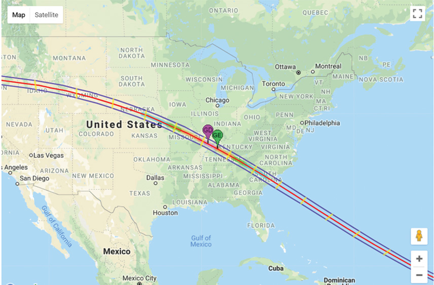
Figure 9.7 Path projection for the total solar eclipse on August 21, 2017
(Source: http://www.weather.gov/lmk/eclipse_2017, accessed August 21, 2018)
On August 21, 2017, North America experienced a total solar eclipse—with possibly the longest path of a total solar eclipse across Earth ever, and certainly the longest across the continent in ninety-nine years. The last eclipse over the United States, in 1979, passed over only a portion of the continent. The NASA trajectory shown in Figure 9.7 for the sun–moon–earth alignment was made using Gauss’s methods, the same ones he invented for tracking the asteroid Ceres. On that Monday in August 2017, the path of the eclipse swept across the continent with startling effect.
You may have seen the eclipse, in either total or partial coverage, depending upon where you were during the event. By happenstance, I was in Columbia, Missouri, that day and experienced a complete covering of the sun. For that brief time, day was night … literally. It was both exciting and terrifying. Realizing what was happening and knowing beforehand that the event would last a mere two minutes, forty seconds at my location—or about forty-five total minutes, including the coming and going phases—made it exhilarating to witness. To be in the presence of such a phenomenon brought to mind the infinitesimally small stature of Earth’s inhabitants compared with astronomical events. For me, there was a feeling of complete lack of control. I do not know about others, as I kept this feeling to myself at the time. Yet, I knew, too, that NASA’s prediction that the eclipse was a passing phenomenon was accurate, because it was based on Gauss’s equations—you know, the ones he proved in 1801 and that have been reliably used innumerable times since. Hence, my uneasy feeling was transitory. I quietly thanked Gauss.
The normal curve is far more prevalent in our lives than just in reporting school-based tests or predicting the weather. As a way of showing a data distribution, it is seemingly ubiquitous in our daily encounters: with print news, on TV, in advertising, when labeling groceries, and much more. Obviously, it is not always presented as a bell-shaped distribution. A pie chart, a bar graph (histogram), and pictographs of all kinds are actually representations of distributional statistics. Almost without effort, we can create myriad such graphs, by using Excel and other programs, or by just drawing one on a napkin to explain something to a friend when having coffee at Starbucks or Costa Coffee. Whether we draw these graphs with a pencil or using a computer program, the mathematics behind them comes from Laplace and Gauss.
The point for us in seeing these as quantification of our worldview is to realize that, prior to Gauss, things were not so methodologically based. Of course, pie charts, histograms, and other pictographs existed before Gauss, as we have described throughout this book (recall that Galileo, in the sixteenth century, recognized distributions of stars and planets and presented them graphically). But these were simple drawings without mathematical support or proofs—just conjectures at the time. They could be used to immediately represent some observed quantity, but, without an underlying architecture, such drawings were not reliable. They could not be used to track stars for mariners’ navigation or to accurately determine the distance between towns, countries, or oceans. It would be silly (nay, dangerous) if NASA’s projections for the flight path of manned and unmanned rockets were done using a seat-of-the-pants drawing. To make things truly useful, the underlying, provable mathematics is needed. Only then can the calculations become reliable estimates with known limits. Gauss’s work established this foundation.
* * * * * *
Yet another real-world example of Gauss’s influence on our daily lives is seen in the devising of driving routes used by carrier companies such as FedEx and UPS. Of course, these companies must deliver consumer goods to the correct address hundreds of thousands of times every day. They employ thousands of drivers, and each one has a unique routing sheet, giving the best street route for that day’s deliveries. Imagine if the drivers’ routes were established by drawing lines on a street map. Chaos! Clearly, a methodology for calculating all the routes is a business necessity. Fortunately, a formula is available from which they can program computers to do the job—a formula invented by Gauss. Even traffic flows can be factored into the algorithm in real time to update each driver on the most efficient course throughout the day.
The story of the American express delivery industry’s founding is legendary. In 1965, Fred Smith, a Yale University undergraduate, got the idea while studying Gauss. He wrote a term paper describing his business model, calling his express delivery company “Federal” because he believed the word evoked patriotism. He received a high mark on the paper—mostly for ingenuity, not usefulness, because his professor thought the idea impractical. Upon graduation, Smith entered the military, but the idea stuck with him. He continued to refine it while in the service; when he completed his tour of duty in 1971, he immediately started up Federal Express, now FedEx.
In the early years of these delivery companies, they used “operations research” (or “OR”) to formulate routes, with variables, such as type of package and time of delivery, being entered into multiple regression equations. Since then, they have evolved their methods to more sophisticated modeling, including a special type called “hierarchical linear modeling” (or “HLM”). All these statistical modeling approaches stem from the foundational work of that sage, Carl Gauss.
Even on a technical level, the relevance of Gaussian methods is still strong. Recently, I was invited to a routine colloquium devoted to “consideration of the computational and statistical issues for high dimensional Bayesian model selection with Gaussian priors.” I am sure Bayes and Gauss would be pleased that their procedures are still the subject of active discussion.
As we see in this chapter, quantification is not just a matter of establishing the formulas—it’s entering our daily lives more and more thoroughly. It has taken a quantum leap forward with the imaginative and groundbreaking work of the semi-reclusive genius of Göttingen, Carl Gauss.