Part II: Sector Analysis

Introduction

This second part has one chapter for each GICS sector. The format of each chapter is the same and is as follows:

• Each chapter begins with the sector’s definition and gives as examples its largest companies.
• Then two following sections correspond to companies in the S&P 500 and the Russell 2000.
• For each reference set, the individually relevant factors are listed and a strategy is proposed. Each strategy is simulated on 15 years without, then with, hedging. The hedging tactics have been previously discussed.
• The performance consistency is evaluated through three, five-year periods, and is followed by a short comment.

There are 10 sectors, therefore 10 chapters, and an eleventh chapter about the Dow Jones Industrial Average. The last chapter of this part compares the strategies with two series of sector ETFs.

Chapter 4: Consumer Discretionary

Sector overview

Definition

The definition given by Morgan Stanley Capital International (MSCI) and Standard & Poor’s in their Global Industry Classification Standard (GICS®) is:

The Consumer Discretionary Sector encompasses those businesses that tend to be the most sensitive to economic cycles. Its manufacturing segment includes automotive, household durable goods, leisure equipment, and textiles & apparel. The services segment includes hotels, restaurants and other leisure facilities, media production and services, and consumer retailing and services.

Companies

This sector contains 84 companies in the S&P 500 and 259 in the Russell 2000, making it the largest for large caps. Table 4.1 gives the 10 largest companies in the sector by market capitalisation at the time of writing. Depending on share price relative moves, the list may have changed when you read this.

Table 4.1: 10 largest companies in the S&P 500 Consumer Discretionary sector

S&P 500 strategy

Individually relevant factors

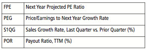
Table 4.2 gives the individually relevant fundamental factors for the S&P 500 Consumer Discretionary segment. What is an “individually relevant” factor has been explained in the Methodology part.

Table 4.2: Individually relevant factors: S&P 500 Consumer Discretionary

Strategy description

I propose a strategy using the Payout Ratio (which is individually relevant) and the Gross Margin (which is not individually relevant, but is relevant in association with other factors).

Table 4.3 provides the strategy summary.

Table 4.3: Strategy description: S&P 500 Consumer Discretionary

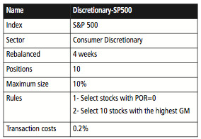
The choice of factors has been made by testing. However, I want to verify that it is a reasonable hypothesis (see my definition of quantitative investing in Part I). In other words, it can be rationalised and interpreted. Here, the interpretation is to select companies that don’t pay a dividend, and have a high gross margin. They are companies more focused on growing their business than on paying shareholders an income.

It may look strange that the individually relevant factor (POR) is used only as a filter, and Gross Margin to rank companies. However simulation shows that the first rule used alone brings an additional annualised return of 3% to the reference set, and the second rule an additional annualised return under 1%. Together, they bring an additional annualised return of 5%. It means that the filter on POR is the primary source of gain.

Basic simulation

The simulation starts in January 1999. The 10 stocks selected at this time are AZO (AutoZone), BIG (Big Lots), CCMO (CC Media Holdings ), CZR (Caesars Entertainment), FTLAQ (Fruit of the Loom), KSS (Kohl’s Corp), KWP (King World Productions), M (Macy’s), MIR (Mirage Resorts), RBK (Reebok International). Each is allotted 10% of the portfolio capital.

Note that four of them have disappeared from the stock market as publicly traded companies: FTLAQ in 2002, KWP in 1999, MIR in 2000, RBK in 2006. However they are taken into account in simulations as long as they have been a part of the S&P 500 Index at one time.

Holdings and allocations are recalculated every four weeks. In case the rebalancing date is a holiday, it is done the next trading day. The buying and selling prices are taken on market opening. As a consequence, the approximation is made that all orders are simultaneous. In this case, “all orders” means two or less: the maximum turnover is 20% and less than 10% on average. S&P 500 companies are very liquid, so it is realistic to think that orders can be filled at open price or very close to it, at least for most individual investors. For a fund with a larger money allocation by holding, techniques can be used to optimise the average cost. I do not address this subject here.

[This short explanation is given as an example to show how it works – this explanation won’t be repeated for the following simulations.]

The total return is 696% (this takes into account transaction costs: about 24% for the whole period if we assume 0.1% per trade). The 61% drawdown is measured between the 2007 top and the 2008 low.

Two quick observations:

1. It would be impossible to obtain the same return by leveraging SPY: a 100% loss would be reached before the 2009 recovery.
2. The strategy recovers faster than the benchmark: it makes a new high as soon as early 2010, whereas SPY makes it in 2013.

It is said that the best fund managers have a Sharpe ratio around 0.8 on periods over a decade (in the real world, not in simulations). So, a Sharpe ratio of 0.44 is not amazing, but it is very good compared with SPY. The fact that the Sortino ratio is higher than the Sharpe ratio is also good: it shows that the deviations from the mean are stronger upward than downward. The risk (standard deviation) is higher than SPY, but it stays in the same 5% range. For a stock strategy, I consider that the correlation with the benchmark is really high above 0.7. Here, at 0.64, it is moderately high. The stock market moves are a prominent factor in the strategy performance, but not overly prominent.

Fig 4.1: Simulation data and equity curve: S&P 500 Consumer Discretionary

NB: due to a graphical issue, there is a gap in the time axis on all charts: all simulations end on 1/1/2014.

Hedged simulation

The data and chart for the hedged simulation are obtained by combining the basic strategy with the hedging described in the previous chapter. All hedged simulations described in this book have been run on the same principle.

The return is much better than the non-hedged version, but the most impressive difference is in the max drawdown: it is divided by more than two (-61% previously, -27% here). Hedging has considerably smoothed market downturns. The Sharpe ratio is good, the Sortino ratio even better. Below 0.5, I consider that the correlation with SPY is low.

Fig 4.2: Simulation data and equity curve: S&P 500 Consumer Discretionary, Hedged

Consistency

To evaluate the consistency over time, here are the annualised returns with hedging over three, five-year periods:

Table 4.4: Consistency over five-year periods

Comment

Consumer Discretionary is a cyclical sector. A protection tactic is necessary to avoid heavy losses in market downturns. Hedging may be a better solution than going to cash to maximise the return and limit the drawdown. This strategy was very profitable with a greater than 30% return during the first five-year period, returns were lower but stayed profitable in the second period, then came back close to 30% in the third period.

It looks a robust strategy for the long term, but Consumer Discretionary stocks are sensitive to economic cycles. As a consequence, the return may vary significantly over shorter terms.

Russell 2000 Strategy

Individually relevant factors

Fundamental indicators often don’t work the same way for small caps and large caps, even in the same sector. The reasons may be due to company size and specific to sectors. As a consequence, the individually relevant factors and strategies are generally found to be different.

Here are the factors from my working list that are individually relevant for the Russell 2000 Consumer Discretionary reference set:

Table 4.5: Individually relevant factors: Russell 2000 Consumer Discretionary

Description

I propose a strategy using the two individually relevant factors in the list. A summary of this strategy is given in Table 4.6.

Table 4.6: Strategy description: Russell 2000 Consumer Discretionary

The rationalised interpretation is to select relatively cheap companies regarding their earnings estimate and free cash flow.

Russell 2000 companies are less liquid, thus a higher figure is used to model the transaction costs.

Basic simulation

I propose an exercise for these charts in Part II: look at the numbers in the screenshots and try to interpret them the same way I did for the first reference set. You may learn much more doing it yourself than reading my interpretation. Here are the main points to look at:

• The annualised return. Every investor has a different idea of what is a good return. Moreover, the return alone makes little sense without looking at the max drawdown and standard deviation. For strategies using a four-week rebalancing, my opinion is that an annualised return is attractive above 20%.
• The max drawdown. In absolute value, each investor must determine an acceptable threshold. I consider that a max drawdown beyond -40% is scary on an individual strategy. When designing a real portfolio combining various strategies, I try to keep it below 20%, knowing that it might be worse in the future.
• The Sharpe and Sortino ratios. In this context I consider that below 0.5 is bad, above 0.8 is good, above 1.5 is very good.
• The standard deviation alone makes little sense without looking at the annualised return. However you can compare it with the benchmark’s standard deviation: here 20% on the period. It gives a limit for separating relatively safe and relatively risky strategies.
• The correlation with the benchmark is not good or bad in itself. But as holding SPY all the time is a very risky strategy, a low correlation should be a positive clue. It is confirmed here: the best strategies in terms of risk-adjusted performance have a low correlation with SPY. Nevertheless, don’t make this a rule in all contexts.

Fig 4.3: Simulation data and equity curve: Russell 2000 Consumer Discretionary

Hedged simulation

Fig 4.4: Simulation data and equity curve: Russell 2000 Consumer Discretionary, hedged

Consistency

Annualised returns with hedging by five-year periods:

Table 4.7: Consistency over five-year periods

Comment

The small cap portfolio magnifies the return and also the risk in terms of drawdown and volatility. Once again, a protection tactic is a must to avoid unacceptable drawdowns. In its hedged versions, the small cap portfolio has a slightly better risk-adjusted return (Sharp and Sortino ratios) than the large cap portfolio. The three, five-year returns show the same cyclical pattern as the S&P 500 strategy, with an even larger amplitude. Small companies are usually more volatile than large caps: they go up faster when the risk appetite leads the market, and they fall harder in a bear market.